Biosignal and Biomedical Image Processing MATLAB based Applications - John L. Semmlow

In the covariance matrix, the diagonals which give the variance of the six signals vary since the amplitudes of the signals are different. The covariance between the first four signals is zero, demonstrating the orthogonality of these signals. The correlation between the 5th and 6th signals and the other sinusoids can be best observed from the correlation matrix:

In the correlation matrix, the correlation of each signal with itself is, of course, 1.0. The 1.5 Hz sine (the 5th column of the data matrix) shows good correlation with the 1.0 and 2.0 Hz cosine (2nd and 4th rows) but not the other sinewaves, while the 1.5 Hz cosine (the 6th column) shows the opposite. Hence, sinusoids that are not harmonically related are not orthogonal and do show some correlation.

SAMPLING THEORY AND FINITE DATA CONSIDERATIONS

To convert an analog waveform into a digitized version residing in memory requires two operations: sampling the waveform at discrete points in time,* and, if the waveform is longer than the computer memory, isolating a segment of the analog waveform for the conversion. The waveform segmentation operation is windowing as mentioned previously, and the consequences of this operation are discussed in the next chapter. If the purpose of sampling is to produce a digitized copy of the original waveform, then the critical issue is how well does this copy represent the original? Stated another way, can the original be reconstructed from the digitized copy? If so, then the copy is clearly adequate. The

*As described in Chapter 1, this operation involves both time slicing, termed sampling, and amplitude slicing, termed quantization.

Copyright 2004 by Marcel Dekker, Inc. All Rights Reserved.

answer to this question depends on the frequency at which the analog waveform is sampled relative to the frequencies that it contains.

The question of what sampling frequency should be used can be best addressed assuming a simple waveform, a single sinusoid.* All finite, continuous waveforms can be represented by a series of sinusoids (possibly an infinite series), so if we can determine the appropriate sampling frequency for a single sinusoid, we have also solved the more general problem. The “Shannon Sampling Theorem” states that any sinusoidal waveform can be uniquely reconstructed provided it is sampled at least twice in one period. (Equally spaced samples are assumed). That is, the sampling frequency, fs, must be ≥ 2fsinusoid. In other words, only two equally spaced samples are required to uniquely specify a sinusoid, and these can be taken anywhere over the cycle. Extending this to a general analog waveform, Shannon’s Sampling Theorem states that a continuous waveform can be reconstructed without loss of information provided the sampling frequency is greater than twice the highest frequency in the analog waveform:

As mentioned in Chapter 1, in practical situations, fmax is usually taken as the highest frequency in the analog waveform for which less than a negligible amount of energy exists.

The sampling process is equivalent to multiplying the analog waveform by a repeating series of short pulses. This repeating series of short pulses is sometimes referred to as the sampling function. Recall that the ideal short pulse is called the impulse function, δ(t). In theory, the impulse function is infinitely short, but is also infinitely tall, so that its total area equals 1. (This must be justified using limits, but any pulse that is very short compared to the dynamics of the sampled waveform will due. Recall the sampling pulse produced in most modern analog-to-digital converters, termed the aperture time, is typically less than 100 nsec.) The sampling function can be stated mathematically using the impulse response.

k=−∞

where Ts is the sample interval and equals 1/fs.

For an analog waveform, x(t), the sampled version, x(n), is given by multiplying x(t) by the sampling function in Eq. (22):

*A sinusoid has a straightforward frequency domain representation: only a single complex point at the frequency of the sinusoid. Classical methods of frequency analysis described in the next chapter make use of this fact.

Copyright 2004 by Marcel Dekker, Inc. All Rights Reserved.

k=−∞

The frequency spectrum of the sampling process represented by Eq. (23) can be determined by taking advantage of fact that multiplication in the time domain is equivalent to convolution in frequency domain (and vice versa). Hence, the frequency characteristic of a sampled waveform is just the convolution of the analog waveform spectrum with the sampling function spectrum. Figure 2.9A shows the spectrum of a sampling function having a repetition rate of Ts, and Figure 2.9B shows the spectrum of a hypothetical signal that has a well-defined maximum frequency, fmax. Figure 2.9C shows the spectrum of the sampled waveform assuming fs = 1/Ts ≥ 2fmax. Note that the frequency characteristic of the sampled waveform is the same as the original for the lower frequencies, but the sampled spectrum now has a repetition of the original spectrum reflected on either side of fs and at multiples of fs. Nonetheless, it would be possible to recover the original spectrum simply by filtering the sampled data by an ideal lowpass filter with a bandwidth > fmax as shown in Figure 2.9E. Figure 2.9D shows the spectrum that results if the digitized data were sampled at fs < 2fmax, in this case fs = 1.5fmax. Note that the reflected portion of the spectrum has become intermixed with the original spectrum, and no filter can unmix them.* When fs < 2fmax, the sampled data suffers from spectral overlap, better known as aliasing. The sampled data no longer provides a unique representation of the analog waveform, and recovery is not possible.

When correctly sampled, the original spectrum can by recovered by applying an ideal lowpass filter (digital filter) to the digitized data. In Chapter 4, we show that an ideal lowpass filter has an impulse response given by:

= sin(2πfcTs n)

h(n) (25)

πn

where Ts is the sample interval and fc is the filter’s cutoff frequency. Unfortunately, in order for this impulse function to produce an ideal filter,

it must be infinitely long. As demonstrated in Chapter 4, truncating h(n) results in a filter that is less than ideal. However if fs >> fmax, as is often the case, then any reasonable lowpass filter would suffice to recover the original waveform, Figure 2.9F. In fact, using sampling frequencies much greater than required is the norm, and often the lowpass filter is provided only by the response characteristics of the output, or display device which is sufficient to reconstruct an adequate looking signal.

*You might argue that you could recover the original spectrum if you knew exactly the spectrum of the original analog waveform, but with this much information, why bother to sample the waveform in the first place!

Copyright 2004 by Marcel Dekker, Inc. All Rights Reserved.

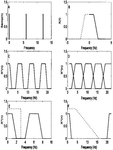
FIGURE 2.9 Consequences of sampling expressed in the frequency domain. (A) Frequency spectrum of a repetitive impulse function sampling at 6 Hz. (B) Frequency spectrum of a hypothetical time signal that has a maximum frequency, fmax, around 2 Hz. (Note negative frequencies occur with complex representation).

(C)Frequency spectrum of sampled waveform when the sampling frequency was greater that twice the highest frequency component in the sampled waveform.

(D)Frequency spectrum of sampled waveform when the sampling frequency was less that twice the highest frequency component in the sampled waveform. Note the overlap. (E) Recovery of correctly sampled waveform using an ideal lowpass filter

(dotted line). (F) Recovery of a waveform when the sampling frequency is much much greater that twice the highest frequency in the sampled waveform (fs = 10fmax). In this case, the lowpass filter (dotted line) need not have as sharp a cutoff.

Copyright 2004 by Marcel Dekker, Inc. All Rights Reserved.

Edge Effects

An advantage of dealing with infinite data is that one need not be concerned with the end points since there are no end points. However, finite data consist of numerical sequences having a fixed length with fixed end points at the beginning and end of the sequence. Some operations, such as convolution, may produce additional data points while some operations will require additional data points to complete their operation on the data set. The question then becomes how to add or eliminate data points, and there are a number of popular strategies for dealing with these edge effects.

There are three common strategies for extending a data set when additional points are needed: extending with zeros (or a constant), termed zero padding; extending using periodicity or wraparound; and extending by reflection, also known as symmetric extension. These options are illustrated in Figure 2.10. In the zero padding approach, zeros are added to the end or beginning of the data sequence (Figure 2.10A). This approach is frequently used in spectral analysis and is justified by the implicit assumption that the waveform is zero outside of the sample period anyway. A variant of zero padding is constant padding, where the data sequence is extended using a constant value, often the last (or first) value in the sequence. If the waveform can be reasonably thought of as one cycle of a periodic function, then the wraparound approach is clearly justified (Figure 2.10B). Here the data are extended by tacking on the initial data sequence to the end of the data set and visa versa. This is quite easy to implement numerically: simply make all operations involving the data sequence index modulo N, where N is the initial length of the data set. These two approaches will, in general, produce a discontinuity at the beginning or end of the data set, which can lead to artifact in certain situations. The symmetric reflection approach eliminates this discontinuity by tacking on the end points in reverse order (or beginning points if extending the beginning of the data sequence) (Figure 2.10C).*

To reduce the number of points in cases where an operation has generated additional data, two strategies are common: simply eliminate the additional points at the end of the data set, or eliminate data from both ends of the data set, usually symmetrically. The latter is used when the data are considered periodic and it is desired to retain the same period or when other similar concerns are involved. An example of this is circular or periodic convolution. In this case, the original data set is extended using the wraparound strategy, convolution is performed on the extended data set, then the additional points are removed

*When using this extension, there is a question as to whether or not to repeat the last point in the extension; either strategy will produce a smooth extension. The answer to this question will depend on the type of operation being performed and the number of data points involved, and determining the best approach may require empirical evaluation.

Copyright 2004 by Marcel Dekker, Inc. All Rights Reserved.

FIGURE 2.10 Three strategies for extending the length of a finite data set. (A) Zero padding: Zeros are added at the ends of the data set. (B) Periodic or wraparound: The waveform is assumed periodic so the end points are added at the beginning, and beginning points are added at the end. (C) Symmetric: Points are added to the ends in reverse order. Using this strategy the edge points may be repeated as was done at the beginning of the data set, or not repeated as at the end of the set.

symmetrically. The goal is to preserve the relative phase between waveforms preand post-convolution. Periodic convolution is often used in wavelet analysis where a data set may be operated on sequentially a number of times, and examples are found in Chapter 7.

PROBLEMS

1. Load the data in ensemble_data.mat found in the CD. This file contains a data matrix labeled data. The data matrix contains 100 responses of a second-

Copyright 2004 by Marcel Dekker, Inc. All Rights Reserved.

order system buried in noise. In this matrix each row is a separate response. Plot several randomly selected samples of these responses. Is it possible to evaluate the second-order response from any single record? Construct and plot the ensemble average for this data. Also construct and plot the ensemble standard deviation.

2.Use the MATLAB autocorrelation and random number routine to plot the autocorrelation sequence of white noise. Use arrays of 2048 and 256 points to show the affect of data length on this operation. Repeat for both uniform and Gaussian (normal) noise. (Use the MATLAB routines rand and randn, respectively.)

3.Construct a 512-point noise arrray then filter by averaging the points three

at a time. That is, construct a new array in which every point is the average of the preceding three points in the noise array: y(n) = 1/3 x(n) + 1/3 x(n − 1) + 1/3 x(n − 2). Note that the new array will be two points shorter than the original noise array. Construct and plot the autocorrelation of this filtered array. You may want to save the output, or the code that generates it, for use in a spectral analysis problem at the end of Chapter 3. (See Problem 2, Chapter 3.)

4.Repeat the operation of Problem 3 to find the autocorrelation, but use convolution to implement the filter. That is, construct a filter function consisting of 3 equal coefficients of 1/3: (h(n) = [1/3 1/3 1/3]). Then convolve this weighting function with the random array using conv.

5.Repeat the process in Problem 4 using a 10-weight averaging filter. (Note that it is much easier to implement such a running average filter with this many weights using convolution.)

6.Construct an array containing the impulse response of a first-order process. The impulse of a first-order process is given by the equation: y(t) = e−t/τ (scaled

for unit amplitude). Assume a sampling frequency of 200 Hz and a time constant, τ, of 1 sec. Make sure the array is at least 5 time constants long. Plot this impulse response to verify its exponential shape. Convolve this impulse response with a 512-point noise array and construct and plot the autocorrelation function of this array. Repeat this analysis for an impulse response with a time constant of 0.2 sec. Save the outputs for use in a spectral analysis problem at the end of Chapter 3. (See Problems 4 and 5, Chapter 3.)

7.Repeat Problem 5 above using the impulse response of a second-order underdamped process. The impulse response of a second-order underdamped system is given by:

y(t) = δ −δ 1 e−δ2πfnt sin(2πfn√1 − δ2t)

Copyright 2004 by Marcel Dekker, Inc. All Rights Reserved.

Use a sampling rate of 500 Hz and set the damping factor, δ, to 0.1 and the frequency, fn (termed the undamped natural frequency), to 10 Hz. The array should be the equivalent of at least 2.0 seconds of data. Plot the impulse response to check its shape. Again, convolve this impulse response with a 512point noise array and construct and plot the autocorrelation function of this array. Save the outputs for use in a spectral analysis problem at the end of Chapter 3. (See Problem 6, Chapter 3.)

8. Construct 4 damped sinusoids similar to the signal, y(t), in Problem 7. Use a damping factor of 0.04 and generate two seconds of data assuming a sampling frequency of 500 Hz. Two of the 4 signals should have an fn of 10 Hz and the other two an fn of 20 Hz. The two signals at the same frequency should be 90 degrees out of phase (replace the sin with a cos). Are any of these four signals orthogonal?

Copyright 2004 by Marcel Dekker, Inc. All Rights Reserved.

3

Spectral Analysis: Classical Methods

INTRODUCTION

Sometimes the frequency content of the waveform provides more useful information than the time domain representation. Many biological signals demonstrate interesting or diagnostically useful properties when viewed in the socalled frequency domain. Examples of such signals include heart rate, EMG, EEG, ECG, eye movements and other motor responses, acoustic heart sounds, and stomach and intestinal sounds. In fact, just about all biosignals have, at one time or another, been examined in the frequency domain. Figure 3.1 shows the time response of an EEG signal and an estimate of spectral content using the classical Fourier transform method described later. Several peaks in the frequency plot can be seen indicating significant energy in the EEG at these frequencies.

Determining the frequency content of a waveform is termed spectral analysis, and the development of useful approaches for this frequency decomposition has a long and rich history (Marple, 1987). Spectral analysis can be thought of as a mathematical prism (Hubbard, 1998), decomposing a waveform into its constituent frequencies just as a prism decomposes light into its constituent colors (i.e., specific frequencies of the electromagnetic spectrum).

A great variety of techniques exist to perform spectral analysis, each having different strengths and weaknesses. Basically, the methods can be divided into two broad categories: classical methods based on the Fourier transform and modern methods such as those based on the estimation of model parameters.

Copyright 2004 by Marcel Dekker, Inc. All Rights Reserved.

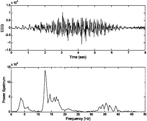
FIGURE 3.1 Upper plot: Segment of an EEG signal from the PhysioNet data bank (Golberger et al.), and the resultant power spectrum (lower plot).

The accurate determination of the waveform’s spectrum requires that the signal be periodic, or of finite length, and noise-free. The problem is that in many biological applications the waveform of interest is either infinite or of sufficient length that only a portion of it is available for analysis. Moreover, biosignals are often corrupted by substantial amounts of noise or artifact. If only a portion of the actual signal can be analyzed, and/or if the waveform contains noise along with the signal, then all spectral analysis techniques must necessarily be approximate; they are estimates of the true spectrum. The various spectral analysis approaches attempt to improve the estimation accuracy of specific spectral features.

Intelligent application of spectral analysis techniques requires an understanding of what spectral features are likely to be of interest and which methods

Copyright 2004 by Marcel Dekker, Inc. All Rights Reserved.