

Biosignal and Biomedical Image Processing MATLAB based Applications - John L. Semmlow
.pdfFIGURE 9.13 Scree plot of eigenvalues from the data set of Figure 9.12. Note the shape break at N = 3, indicating that there are only three independent variables in the data set of five waveforms. Hence, the ICA algorithm will be requested to search for only three components.
% |
|
% Do PCA and plot Eigenvalues |
|
figure; |
|
[U,S,pc]= svd(X,0); |
% Use single value decomposition |
eigen = diag(S).v2; |
% Get the eigenvalues |
plot(eigen,’k’); |
% Scree plot |
......labels and title..........
%
nu_ICA = input(’Enter the number of independent components’);
% Compute ICA
W = jadeR(X,nu_ICA); |
% Determine the mixing matrix |
ic = (W * X)’; |
% Determine the IC’s from the |
|
% mixing matrix |
figure; |
% Plot independent components |
plot(t,ic(:,1)-4,’k’,t,ic(:,2),’k’,t,ic(:,3) 4,’k’);
......labels and title..........
The original source signals are shown in Figure 9.12. These are mixed together in different proportions to produce the five signals shown in Figure 9.14. The Scree plot of the eigenvalues obtained from the five-variable data set does show a marked break at 3 suggesting that there, in fact, only three separate components, Figure 9.13. Applying ICA to the five-variable mixture in Figure
Copyright 2004 by Marcel Dekker, Inc. All Rights Reserved.
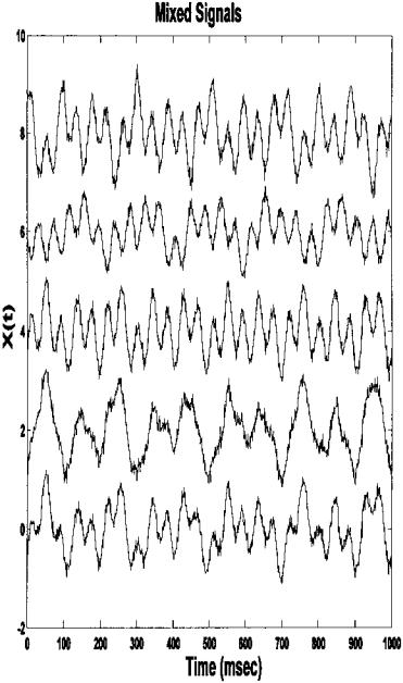
FIGURE 9.14 Five signals created by mixing three different waveforms and noise. ICA was applied to this data set to recover the original signals. The results of applying ICA to this data set are seen in Figure 9.15.
Copyright 2004 by Marcel Dekker, Inc. All Rights Reserved.
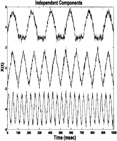
FIGURE 9.15 The three independent components found by ICA in Example 9.3. Note that these are nearly identical to the original, unmixed components. The presence of a small amount of noise does not appear to hinder the algorithm.
9.14 recovers the original source signals as shown in Figure 9.15. This figure dramatically demonstrates the ability of this approach to recover the original signals even in the presence of modest noise. ICA has been applied to biosignals to estimate the underlying sources in an multi-lead EEG signal, to improve the detection of active neural areas in functional magnetic resonance imaging, and to uncover the underlying neural control components in an eye movement motor control system. Given the power of the approach, many other applications are sure to follow.
Copyright 2004 by Marcel Dekker, Inc. All Rights Reserved.
PROBLEMS
1. Load the two-variable data set, X, contained in file p1_data. Assume for plotting that the sample frequency is 500 Hz. While you are not given the dimensions or orientation of the data set, you can assume the number of time samples is much greater than the number of measured signals.
(A) Rotate these data by an angle entered through the keyboard and output the covariance (from the covariance matrix) after each rotation. Use the function rotate to do the rotation. See comments in the function for details. Continue to rotate the data set manually until the covariances are very small (less than 10-4). Plot the rotated and unrotated variables as a scatter plot and output their variances (also from covariance matrix). The variances will be the eigenvalues found by PCA and the rotated data the principal components.
(B)Now apply PCA using the approach given in Example 9.1 and compare the scatter plots with the manually rotated data. Compare the variances of the principal components from PCA (which can be obtained from the eigenvalues) with the variances obtained by manual rotation in (A) above.
2.Load the multi-variable data set, X, contained in file p2_data. Make the same assumptions with regard to sampling frequency and data set size as in Problem 1 above.
(A)Determine the actual dimension of the data using PCA and the scree plot.
(B)Perform an ICA analysis using either the Jade or FastICA algorithm limiting the number of components determined from the scree plot. Plot independent components.
Copyright 2004 by Marcel Dekker, Inc. All Rights Reserved.