Biosignal and Biomedical Image Processing MATLAB based Applications - John L. Semmlow

%Define projective transformation Vary offset up to Max_tilt offset = Max_tilt*N*i/Nu_frame;

X = [1 offset 1 offset; 1-offset M-offset; N offset ...

M-offset; N-offset...1 offset]; Tform2 = maketform(’projective’, U, X);

[I_proj(:,:,1,i), map] = gray2ind(imtransform(I,Tform2,...

’Xdata’,[1 N],’Ydata’,[1 M]));

% Make image tilt back and forth I_proj(:,:,1,2*Nu_frame 1-i) = I_proj(:,:,1,i);

end

%

% Display first 12 images as a montage montage(I_proj(:,:,:,1:12),map);

While it is not possible to show the movie that is produced by this code, the various frames are shown as a montage in Figure 11.12. The last three problems in the problem set explore the use of spatial transformations used in combination to make movies.

IMAGE REGISTRATION

Image registration is the alignment of two or more images so they best superimpose. This task has become increasingly important in medical imaging as it is used for merging images acquired using different modalities (for example, MRI and PET). Registration is also useful for comparing images taken of the same structure at different points in time. In functional magnetic resonance imaging (fMRI), image alignment is needed for images taken sequentially in time as well as between images that have different resolutions. To achieve the best alignment, it may be necessary to transform the images using any or all of the transformations described previously. Image registration can be quite challenging even when the images are identical or very similar (as will be the case in the examples and problems given here). Frequently the images to be aligned are not that similar, perhaps because they have been acquired using different modalities. The difficulty in accurately aligning images that are only moderately similar presents a significant challenge to image registration algorithms, so the task is often aided by a human intervention or the use of embedded markers for reference.

Approaches to image registration can be divided into two broad categories: unassisted image registration where the algorithm generates the alignment without human intervention, and interactive registration where a human operator

Copyright 2004 by Marcel Dekker, Inc. All Rights Reserved.

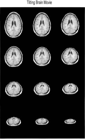
FIGURE 11.12 Montage display of the movie produced by the code in Example 11.7. The various projections give the appearance of the brain slice tilting and moving back in space. Only half the 24 frames are shown here as the rest are the same, just presented in reverse order to give the appearance of the brain rocking back and forth. (Original image from the MATLAB Image Processing Toolbox. Copyright 1993–2003, The Math Works, Inc. Reprinted with permission.)

Copyright 2004 by Marcel Dekker, Inc. All Rights Reserved.

guides or aids the registration process. The former approach usually relies on some optimization technique to maximize the correlation between the images. In the latter approach, a human operator may aid the alignment process by selecting corresponding reference points in the images to be aligned: corresponding features are identified by the operator and tagged using some interactive graphics procedure. This approach is well supported in MATLAB’s Image Processing Toolbox. Both of these approaches are demonstrated in the examples and problems.

Unaided Image Registration

Unaided image registration usually involves the application of an optimization algorithm to maximize the correlation, or other measure of similarity, between the images. In this strategy, the appropriate transformation is applied to one of the images, the input image, and a comparison is made between this transformed image and the reference image (also termed the base image). The optimization routine seeks to vary the transformation in some manner until the comparison is best possible. The problem with this approach is the same as with all optimization techniques: the optimization process may converge on a sub-optimal solution (a so-called local maximum), not the optimal solution (the global maximum). Often the solution achieved depends on the starting values of the transformation variables. An example of convergence to a sub-optimal solution and dependency on initial variables is found in Problem 8.

Example 11.8 below uses the optimization routine that is part of the basic MATLAB package, fminsearch (formerly fmins). This routine is based on the simplex (direct search) method, and will adjust any number of parameters to minimize a function specified though a user routine. To maximize the correspondence between the reference image and the input image, the negative of the correlation between the two images is minimized. The routine fminsearch will automatically adjust the transformation variables to achieve this minimum (remember that this may not be the absolute minimum).

To implement an optimization search, a routine is required that applies the transformation variables supplied by fminsearch, performs an appropriate trial transformation on the input image, then compares the trial image with the reference image. Following convergence, the optimization routine returns the values of the transformation variables that produce the best comparison. These can then be applied to produce the final aligned image. Note that the programmer must specify the actual structure of the transformation since the optimization routine works blindly and simply seeks a set of variables that produces a minimum output. The transformation selected should be based on the possible mechanisms for misalignment: translations, size changes, rotations, skewness, projective misalignment, or other more complex distortions. For efficiency, the transformation should be one that requires the least number of defining vari-

Copyright 2004 by Marcel Dekker, Inc. All Rights Reserved.

ables. Reducing the number of variables increases the likelihood of optimal convergence and substantially reduces computation time. To minimize the number of transformation variables, the simplest transformation that will compensate for the possible mechanisms of distortions should be used.*

Example 11.8 This is an example of unaided image registration requiring an affine transformation. The input image, the image to be aligned, is a distorted version of the reference image. Specifically, it has been stretched horizontally, compressed vertically, and tilted, all using a single affine transformation. The problem is to find a transformation that will realign this image with the reference image.

Solution MATLAB’s optimization routine fminsearch will be used to determine an optimized transformation that will make the two images as similar as possible. MATLAB’s fminsearch routine calls the user routine rescale to perform the transformation and make the comparison between the two images. The rescale routine assumes that an affine transformation is required and that only the horizontal, vertical, and tilt dimensions need to be adjusted. (It does not, for example, take into account possible translations between the two images, although this would not be too difficult to incorporate.) The fminsearch routine requires as input arguments, the name of the routine whose output is to be minimized (in this example, rescale), and the initial values of the transformation variables (in this example, all 1’s). The routine uses the size of the initial value vector to determine how many variables it needs to adjust (in this case, three variables). Any additional input arguments following an optional vector specifying operational features are passed to rescale immediately following the transformation variables. The optimization routine will continue to call rescale automatically until it has found an acceptable minimum for the error (or until some maximum number of iterations is reached, see the associated help file).

%Example 11.8 and Figure 11.13

%Image registration after spatial transformation

%Load a frame of the MRI image (mri.tif). Transform the original

%image by increasing it horizontally, decreasing it vertically,

%and tilting it to the right. Also decrease image contrast

%slightly

%Use MATLAB’s basic optimization routine, ’fminsearch’ to find

%the transformation that restores the original image shape.

*The number of defining variables depends on the transformation. For example rotation alone only requires one variable, linear transformations require two variables, affine transformations require 3 variables while projective transformations require 4 variables. Two additional variables are required for translations.

Copyright 2004 by Marcel Dekker, Inc. All Rights Reserved.

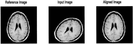
FIGURE 11.13 Unaided image registration requiring several affine transformations. The left image is the original (reference) image and the distorted center image is to be aligned with that image. After a transformation determined by optimization, the right image is quite similar to the reference image. (Original image from the same as fig 11.12.)

.......load mri.tif, frame 18.......

[M N]= size(I);

H_scale = H_scale * N/2; % Convert percent scale to pixels V_scale = V_scale * M;

tilt = tilt * N

%

% Construct distorted image.

Tform = maketform(’affine’, U, X);

I_transform = (imtransform(I,Tform,’Xdata’,[1 N], ...

’Ydata’, [1 M]))*.8;

%

% Now find transformation to realign image initial_scale = [1 1 1]; % Set initial values

[scale,Fval] = fminsearch(’rescale’,initial_scale,[ ], ...

% Realign image using optimized transform

Copyright 2004 by Marcel Dekker, Inc. All Rights Reserved.

X = [1 scale(1) scale(3) 1 scale(2); 1 scale(1) M; ...

N-scale(1) M];

Tform = maketform(’affine’, U, X);

I_aligned = imtransform(I_transform,Tform,’Xdata’,[1 N],

’Ydata’,[1 M]);

%

subplot(1,3,1); imshow(I); %Display the images title(’Original Image’);

subplot(1,3,2); imshow(I_transform); title(’Transformed Image’);

subplot(1,3,3); imshow(I_aligned); title(’Aligned Image’);

The rescale routine is used by fminsearch. This routine takes in the transformation variables supplied by fminsearch, performs a trial transformation, and compares the trial image with the reference image. The routine then returns the error to be minimized calculated as the negative of the correlation between the two images.

function err = rescale(scale, I, I_transform);

%Function used by ’fminsearch’ to rescale an image

%horizontally, vertically, and with tilt.

%Performs transformation and computes correlation between

%original and newly transformed image.

%Inputs:

%Outputs:

%Negative correlation between original and transformed image.

[M N]= size(I);

U = [1 1; 1 M; N M]; % Input triangle

%

% Perform trial transformation

X = [1 scale(1) scale(3) 1 scale(2); 1 scale(1) M; ...

N-scale(1) M];

Tform = maketform(’affine’, U, X);

I_aligned = imtransform(I_transform,Tform,’Xdata’, ...

[1 N], ’Ydata’,[1 M]);

%

% Calculate negative correlation err = -abs(corr2(I_aligned,I));

The results achieved by this registration routine are shown in Figure 11.13. The original reference image is shown on the left, and the input image

Copyright 2004 by Marcel Dekker, Inc. All Rights Reserved.

is in the center. As noted above, this image is the same as the reference except that it has been distorted by several affine transformations (horizontal scratching, vertical compression, and a tilt). The aligned image achieved by the optimization is shown on the right. This image is very similar to the reference image. This optimization was fairly robust: it converged to a correlation of 0.99 from both positive and negative initial values. However, in many cases, convergence can depend on the initial values as demonstrated in Problem 8. This program took about 1 minute to run on a 1 GHz PC.

Interactive Image Registration

Several strategies may be used to guide the registration process. In the example used here, registration will depend on reference marks provided by a human operator. Interactive image registration is well supported by the MATLAB Image Processing Toolbox and includes a graphically based program, cpselect, that automates the process of establishing corresponding reference marks. Under this procedure, the user interactively identifies a number of corresponding features in the reference and input image, and a transform is constructed from these pairs of reference points. The program must specify the type of transformation to be performed (linear, affine, projective, etc.), and the minimum number of reference pairs required will depend on the type of transformation. The number of reference pairs required is the same as the number of variables needed to define a transformation: an affine transformation will require a minimum of three reference points while a projective transformation requires four variables. Linear transformations require only two pairs, while other more complex transformations may require six or more point pairs. In most cases, the alignment is improved if more than the minimal number of point pairs is given.

In Example 11.9, an alignment requiring a projective transformation is presented. This Example uses the routine cp2tform to produce a transformation in Tform format, based on point pairs obtained interactively. The cp2tform routine has a large number of options, but the basic calling structure is:

Tform = cp2tform(input_points, base_points, ‘type’);

where input_points is a m by 2 matrix consisting of x,y coordinates of the reference points in the input image; base_points is a matrix containing the same information for the reference image. This routine assumes that the points are entered in the same order, i.e., that corresponding rows in the two vectors describe corresponding points. The type variable is the same as in maketform and specifies the type of transform (‘affine’, ‘projective’, etc.). The use of this routine is demonstrated in Example 11.9.

Example 11.9 An example of interactive image registration. In this example, an input image is generated by transforming the reference image with a

Copyright 2004 by Marcel Dekker, Inc. All Rights Reserved.

projective transformation including vertical and horizontal translations. The program then opens two windows displaying the reference and input image, and takes in eight reference points for each image from the operator using the MATLAB ginput routine. As each point is taken it, it is displayed as an ‘*’ overlaid on the image. Once all 16 points have been acquired (eight from each image), a transformation is constructed using cp2tform. This transformation is then applied to the input image using imtransform. The reference, input, and realigned images are displayed.

%Example 11.9 Interactive Image Registration

%Load a frame of the MRI image (mri.tif) and perform a spatial

%transformation that tilts the image backward and displaces

%it horizontally and vertically.

%Uses interactive registration and the MATLAB function

%‘cp2tform’ to realign the image

.......Load mri.tif, frame 18 .......

[M N]= size(I);

%

% Construct input image. Perform projective transformation

N-offset H M-offset-V;...N offset H 1 offset-V]; Tform1 = maketform(’projective’, U, X);

I_transform = imtransform(I,Tform1,’Xdata’,[1 N], ...

’Ydata’, [1 M]);

%

%Acquire reference points

%First open two display windows fig(1) = figure;

imshow(I); fig(2) = figure;

imshow(I_transform);

Copyright 2004 by Marcel Dekker, Inc. All Rights Reserved.

title(’Enter four reference points’); for j = 1:nu_points

[x(j,i), y(j,i)] = ginput(1); % Get reference point

%Construct transformation with cp2tform and implement with

%imtransform

%

[Tform2, inpts, base_pts] = cp2tform([x(:,2) y(:,2)], ...

[x(:,1) y(:,1)],’projective’);

I_aligned = imtransform(I_transform,Tform2,’Xdata’, ...

[1 N],’Ydata’,[1 M]);

%

figure;

subplot(1,3,1); imshow(I); % Display the images title(’Original’);

subplot(1,3,2); imshow(I_transform); title(’Transformation’);

subplot(1,3,3); imshow(I_aligned); title(’Realigned’);

The reference and input windows are shown along with the reference points selected in Figure 11.14A and B. Eight points were used rather than the minimal four, because this was found to produce a better result. The influence of the number of reference point used is explored in Problem 9. The result of the transformation is presented in Figure 11.15. This figure shows that the realignment was less that perfect, and, in fact, the correlation after alignment was only 0.78. Nonetheless, the primary advantage of this method is that it couples into the extraordinary abilities of human visual identification and, hence, can be applied to images that are only vaguely similar when correlationbased methods would surely fail.

PROBLEMS

1.Load the MATLAB test pattern image testpat1.png used in Example

11.5.Generate and plot the Fourier transform of this image. First plot only the

25points on either side of the center of this transform, then plot the entire function, but first take the log for better display.

2.Load the horizontal chirp pattern shown in Figure 11.1 (found on the disk as imchirp.tif) and take the Fourier transform as in the above problem. Then multiply the Fourier transform (in complex form) in the horizontal direction by

Copyright 2004 by Marcel Dekker, Inc. All Rights Reserved.

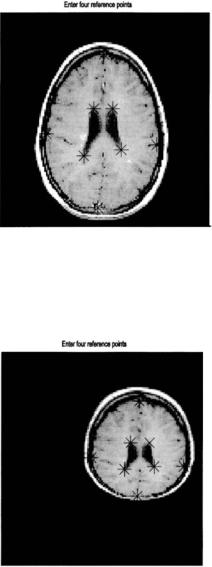
FIGURE 11.14A A reference image used in Example 11.9 showing the reference points as black. (Original image from the MATLAB Image Processing Toolbox. Copyright 1993–2003, The Math Works, Inc. Reprinted with permission.)

FIGURE 11.14B Input image showing reference points corresponding to those shown in Figure 11.14A.

Copyright 2004 by Marcel Dekker, Inc. All Rights Reserved.