Kluwer - Handbook of Biomedical Image Analysis Vol

Figure 9.34: Results on synthetic image with noise variance, σ 2 = 500 using GSM method. Row 5, left: After assign ID (K = 1). Row 5, right: After assign ID (K > 1). Row 6, left: After region to boundary (K = 1). Row 6, right: After region to boundary (K > 1). Row 7, left: Overaly generation with and without crescent moon. Row 8, right: Overaly generation with and wihout crescent moon.

9.5Performance Evaluation System: Rulers and Error Curves

The polyline distance Ds(B1 : B2) between two polygons representing boundary

B1 and B2 is symmetrically defined as the average distance between a vertex of one polygon and the boundary of the other polygon. To define this measure precisely, we first need to define a distance d(v, s) between a point v and a line segment s. The distance d(v, s) between a point v having coordinates (x0, y0), and a line segment having end points (x1, y1) and (x2, y2) is

where

d1 = (x0 − x1)2 + (y0 − y1)2

d2 = (x0 − x2)2 + (y0 − y2)2

(x2 − x1)2 + (y2 − y1)2

The distance db(v, B2) measuring the polyline distance from vertex v to the boundary B2 is defined by

The distance dvb(B1, B2) between the vertices of polygon B1 and the sides of polygon B2 is defined as the sum of the distances from the vertices of the polygon

B1 to the closest side of B2.

ertices B

Reversing the computation from B2 to B1, we can similarly compute dvb(B2, B1). Using Eq. (9.20), the polyline distance between polygons, Ds(B1 : B2) is defined by

dvb(B1, B2) + dvb(B2, B1)

Ds(B1 : B2) = (9.21) (# vertices B1 + # vertices B2)

9.5.1 Mean Error (eNFPpoly)

Using the definition of the polyline distance between two polygons, we can now compute the mean error of the overall system. It is denoted by eNFPpoly and defined

by

where Ds(Gnt , Cnt ) is the polyline distance between the ground truth Gnt and computer-estimated polygons Cnt for patient study n and slice number t. Using the definition of the polyline distance between two polygons, the standard deviation can be computed as

σNFPpoly =

(9.23)

9.5.2Error per Vertex and Error per Arc Length for Bias Computation

Using the polyline distance formulaes, we can compute the error per vertex from one polygon (ground truth) to another polygon (computer estimated). This is defined as the mean error for a vertex v over all the patients and all the slices. The error per vertex for a fixed vertex v when computed between ground truth and computer-estimated boundary is defined by

×

Similary we can compute the error per vertex between computer estimated and ground truth using Eq.(9. 20) Error per arc length is computed in the following

way: For the values evGC where v = 1, 2, 3, . . . , P1, we construct a curve f GC defined on the interval [0,1] which takes the value evGC at point x which is the normalized arc length to vertex v and whose in between values are defined by linear interpolation. We compute the curve f C G between computer estimated boundary and ground truth boundary in a similar way. We then add algebraically

9.5.3 Performance of Synthetic System: Error Curves

9.5.3.1 Small Noise Protocols

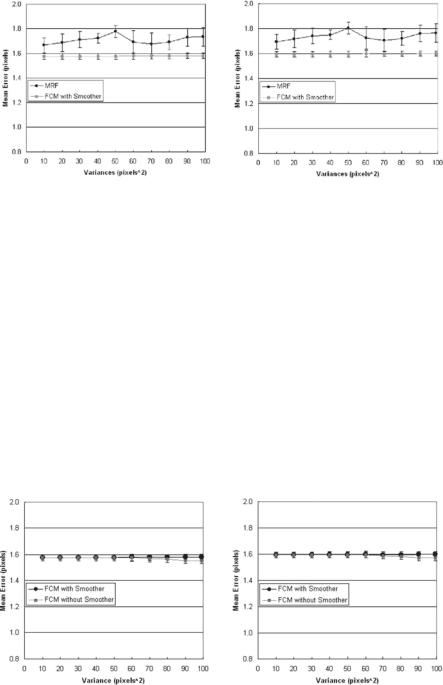
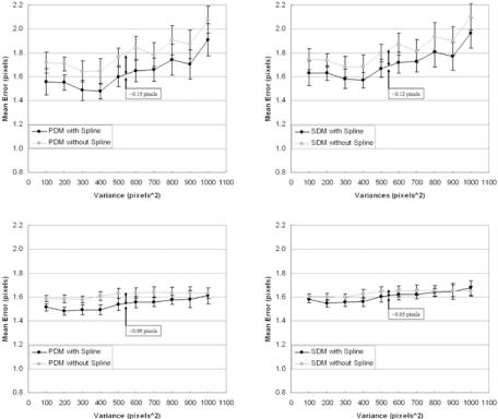
Figure 9.35 (left and right) shows the performance of the synthetic system for the small noise protocol using polyline (see section 9.5) and shortest distance methods. Figure 9.35 (left) compares the mean error curves of the MRF vs. FCM (with smoother) using the PDM, while Fig. 9.35 (right) compares the mean error curves of the MRF vs. FCM (with smoother) using the shortest distance method. Using PDM, as the variance of the noise (σ 2) increases from 0 to 100, the mean error in both methods increases gradually. The mean error for the FCM (with smoother) remains under 1.6 pixels, while the mean error for MRF ranges between 1.6 and 1.8 pixels. The same pattern is observed using SDM method (see Fig. 9.35, right). It is also seen in the two graphs that FCM using PDM has a lower error compared to FCM using SDM.

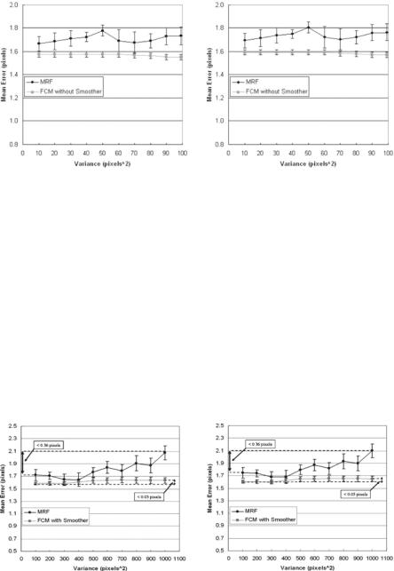
In another procotol, we run the same PDM and SDM for FCM methods but with and without the Perona–Malik smoothing process. This can be seen in Fig. 9.36 (left and right). The method of PDE-based smoothing system improves

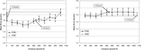
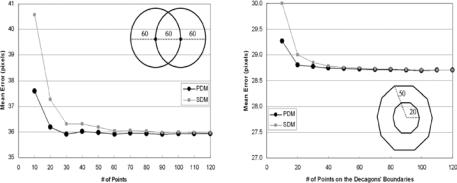
Figure 9.41: Sampling protocol test: Left: Shape optimization test. Right: Concentric shape decagon test. Two circle contours each of radius 60 pixels have their centers separated by 60 pixels. The mean errors given by the PDM and the SDM are plotted against the number of points on the circular contours. As the number of points on each of the contours increases, the difference in the mean errors decreases, and both errors approach an actual value.

points increases on the boundary, the boundary becomes more smooth, but we do not know as to how many points are necessary on the boundary to represent the best lumen shape. Figure 9.41 (left and right) demonstrates the mean error around the boundary versus the number of points on the lumen boundary. As the number of points increases from 10 to 120, the mean error drops rapidly using PDM and SDM methods. Using PDM, the mean error drops rapidly when the number of boundary points increases from 10 to 30 and reaches a stage of convergence when the number of points is 50. The same pattern is observed using the SDM method and the mean error falls rapidly from points 10 to 50 and reaches a stage of convergence when the number of points on the boundary is 80. The stage of convergence here means that there is no more change in the mean error, if the number of points increases beyond a certain limit. Lastly, the fall of the errors as the number of points increases is more rapid for SDM compared to that of PDM, and the starting error (when total points are 10) in SDM is much larger compared to that of PDM. A similar experiment was done synthetically when the boundaries are concentric shapes. We took a simple shape of a concentric decagon (with radius 20 and 50 pixels) and increasing the number of points from 10 to 120. Since the boundaries were concentric, the

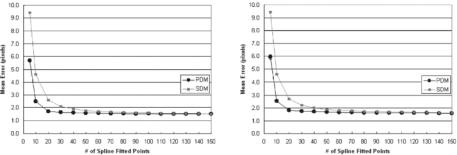
Figure 9.43: Optimization curves. Left: σ 2 = 500. Right: σ 2 = 1000.

fitting splines over the estimated boundaries. There are four parts in this figure showing the effect of splines over two classification systems, using two distance methods: (a) MRF using PDM, (b) MRF using SDM, (c) FCM using PDM, and (d) FCM using SDM. In all four subprotocols, we find the same behavior that the spline-fitted mean errors are lower than nonspline-fitted mean errors. We also observed that there is a very consistent standard deviation error for all four subprotocols. We also did lumen shape optimization on fitted spline shapes, and this can be seen in Fig. 9.43 (left and right). As the number of points on the boundary increases, the mean error drops and reaches a stage of convergence.

9.6 Real Data Analysis: Circular Vs. Elliptical

9.6.1 Circular Binarization

Select class is used for binarization of the classified image. The frequency of each pixel value in the ROI is determined. The core class C0 is the class with the greatest number of pixels. The number of pixels is equivalent to the area of the core. The average area of the entire lumen core is determined from the ground truth boundaries, and this area is compared to the area of the C0 area. A threshold function is used to determine whether to binarize the C0 region, or to merge C0 with C1 and then binarize. We now discuss the methods to compute the average lumen area, lumen core area, and the difference of these, and their comparison.