

Kluwer - Handbook of Biomedical Image Analysis Vol
.2.pdf532 |
Sato |
that underlies the discrete sample data. Second-order local structures around a point of interest in the underlying continuous function can be fully represented using up to second derivatives at the point, that is, the gradient vector and Hessian matrix. In order to reduce noise as well as deal with second-order local structures of “various sizes,” isotropic Gaussian smoothing with different standard deviation (SD) values is combined with derivative computation. Combining Gaussian smoothing has another effect that accurate derivative computation of the Gaussian smoothed version of the underlying “continuous” function is possible by convolution operations within a size-limited local window.
In this chapter, the following topics are discussed:
Multiscale enhancement filtering of second-order local structures, that is, line, sheet, and blob structures [5, 7, 11] in volume data.
Analysis of filter responses for line structures using mathematical line models [7].
Description and quantification (width and orientation measurement) of these local structures [10, 12].
Analysis of sheet width quantification accuracy restricted by imaging resolution [17, 18].
For the multiscale enhancement, we design 3-D enhancement filters, which selectively respond to the specific type of local structures with specific size, based on the eigenvalues of the Hessian matrix of the Gaussian smoothed volume intensity function. The conditions that the eigenvalues need to satisfy for the local structures are analyzed to derive similarity measures to the local structures. We also design a multiscale integration scheme of the filter responses at different Gaussian SD values. The condition for the scale interval is analyzed to enhance equally over a specific range of structure sizes.
For the analysis of filter responses, mathematical line models with a noncircular cross section are used. The basic characteristics of the filter responses and their multiscale integration are analyzed simulationally. Although the line structure is considered here, the presented basic approach is applicable to filter responses to other local structures.
For the detection and quantification, we formulate a method using a secondorder polynomial describing the local structures. We focus on line and sheet structures, which are basically characterized by their medial elements (medial surfaces and axes, respectively) and widths associated with the medial
Hessian-Based Multiscale Enhancement and Segmentation |
533 |
elements. A second-order polynomial around a point of interest is defined by the gradient vector and Hessian matrix at the point. The medial elements are detected based on subvoxel localization of local maximum of the second-order polynomial within the voxel territory of a point of interest. The widths are measured along normal directions of the detected medical elements.
For the analysis of quantification accuracy, a theoretical approach is presented based on mathematical models of imaged local structures, imaging scanners, and quantification processes. Although the sheet structure imaged by MR scanners is focused here, the presented basic approach is applicable to accuracy analysis for different local structures imaged by either MR or CT scanners.
10.2 Multiscale Enhancement Filtering
10.2.1 Measures of Similarity to the Local Structures
Let f (x") be an intensity function of a volume, where x" = (x, y, z). Its Hessian matrix 2 f is given by
|
2 |
f (x) |
|
|
fxx(x") |
fxy(x") |
fxz(x") |
, |
(10.1) |
|
= |
fyx(x) |
fyy(x) |
fyz(x) |
|||||
|
" |
|
" |
" |
" |
|
|
||
|
|
|
|
fzx(x) |
fzy(x) |
fzz(x) |
|
||
|
|
|
|
|
" |
" |
" |
|
|
where |
partial second derivatives of |
f |
( |
) are represented as |
fxx |
( |
) |
= |
∂2 |
f |
( ), |
||
|
|||||||||||||
|
2 |
|
|
x" |
|
x" |
∂ x2 |
x" |
|||||
fyz(x") = |
∂ |
f (x"), and so on. The Hessian matrix 2 f (x"0) at x"0 describes the |
|||||||||||
∂ y∂ z |
|||||||||||||
second-order variations around x0 [3–8, 11–14, 19]. The rotational invariant measures of the second-order local structure can be derived through the eigenvalue analysis of 2 f (x"0).
Let the eigenvalues of 2 f (x") be λ1(x"), λ2(x"), λ3(x") (λ1(x") ≥ λ2(x") ≥ λ3(x")), and their corresponding eigenvectors be e"1(x"), e"2(x"), e"3(x"), respectively. The eigenvector e"1, corresponding to the largest eigenvalue λ1, represents the direction along which the second derivative is maximum, and λ1 gives the maximum second-derivative value. Similarly, λ3 and e"3 give the minimum directional second-derivative value and its direction, and λ2 and e"2 the minimum directional second-derivative value orthogonal to e"3 and its direction, respectively. λ2 and e"2 also give the maximum directional second-derivative value orthogonal to e"1 and its direction.
λ1, λ2, and λ3 are invariant under orthonormal transformations. λ1, λ2, and
λ3 are combined and associated with the intuitive measures of similarity to

534 |
Sato |
Table 10.1: Basic conditions for each local structure and
representative anatomical structures. Each structure is assumed to
be brighter than the surrounding region
Structure |
Eigenvalue condition |
Decomposed condition |
Example(s) |
|||||
|
|
|
|
|
|
|
|
|
Sheet |
λ3 |
λ2 |
λ1 |
0. |
λ3 0 |
|
Cortex |
|
|
|
|
|
|
λ3 λ2 |
0 |
Cartilage |
|
|
|
|
|
|
λ3 λ1 |
0 |
|
|
Line |
λ3 |
λ2 λ1 |
0. |
λ3 0 |
|
Vessel |
||
|
|
|
|
|
λ3 |
λ2 |
|
Bronchus |
|
|
|
|
|
λ2 λ1 |
0 |
|
|
Blob |
λ3 |
λ2 |
λ1 0. |
λ3 |
0 |
|
Nodule |
|
|
|
|
|
|
λ3 |
λ2 |
|
|
|
|
|
|
|
λ2 |
λ1 |
|
|
|
|
|
|
|
|
|
|
|
local structures. Three types of second-order local structures—sheet, line, and blob—can be classified using these eigenvalues. The basic conditions of these local structures and examples of anatomical structures that they represent are summarized in Table 10.1, which shows the conditions for the case where structures are bright in contrast with surrounding regions. Conditions can be similarly specified for the case where the contrast is reversed. Based on these conditions, measures of similarity to these local structures can be derived. With respect to the case of a line, we have already proposed a line filter that takes an original volume f into a volume of a line measure [7] given by
Sline{ |
f |
} = |
|λ3| · ψ (λ2; λ3) · ω(λ1; λ2) λ3 ≤ λ2 < 0 |
(10.2) |
||||||
|
0, |
|
|
|
|
|
otherwise, |
|
||
where ψ is a weight function written as |
|
|
|
|||||||
|
|
|
s |
t |
) |
= |
0 |
|
otherwise, |
(10.3) |
|
|
|
ψ (λ |
; λ |
|
( λt ) |
γst |
λt ≤ λs < 0 |
||
|
|
|
|
|
|
|
λs |
|
|
|
in which γst controls the sharpness of selectivity for the conditions of each local structure (Fig. 10.1(a)), and ω is written as
|
|
|
(1 + |
|
λs |
) |
γst |
λt ≤ λs ≤ 0 |
|
|||||
|
|
|
|λt | |
|
|
|
||||||||
ω(λs; λt ) |
= |
(1 |
− |
α |
λs |
|
)γst |
|λt | > λ |
s |
> 0 |
(10.4) |
|||
|
|
|||||||||||||
|
|
|
|
|λt | |
|
α |
|
|
||||||
|
|
|
|
|
|
|
|
|
|
|
|
|
|
|
|
|
|
|
|
|
|
|
|
|
|
|
|
|
|
|
|
|
0 |
|
|
|
|
|
|
|
otherwise, |
|
||
|
|
|
|
|
|
|
|
|
|
|
|
|
|
|

536 Sato
|
|
e1 |
|
|
|
|
|
|
|
|
|
e3 |
|
|
|
|
e1 |
|
|
|
|
e2 |
|
|
Sheet |
|
e3 |
|
Sheet |
|
|
|
λ3 << λ2 = 0 |
|
|
||||
|
|
|
ψ → 0 |
|
e2ψ → 0 |
λ3 << λ2 = 0 |
|||
|
|
|
|
|
|
||||
|
|
Line |
|
|
|
|
|
||
|
|
|
|
|
|
Blob |
|
|
|
|
|
λ3 = λ2 |
|
|
|
|
|
|
|
Stenosis |
|
|
|
Blob |
|
λ3 = λ2 |
|
|
|
|
|
|
|
|
|
|
|||
λ1 >> 0 |
|
λ2 << λ1 = 0 |
|
λ2 = λ1 << 0 |
|
|
Line |
||
ω → 0 in |
ω → 0 in |
|
λ2 = λ1 |
|
|||||
|
|
|
|
|
ψ → 0 |
λ2 << λ1 = 0 |
|||
|
positive domain |
negative domain |
|
||||||
|
|
(a) |
|
|
|
|
|
(b) |
|
|
|
|
e1 |
|
e3 |
|
|
|
|
|
|
|
|
|
|
|
|
|
|
Groove |
|
|
|
e2 |
|
Blob |
|
|
|
|
|
|
λ3 |
= λ1 << 0 |
|
|
|||
λ1 >> 0 |
|
|
|
|
|
|
|||
|
|
|
Sheet |
|
|
|
|
|
|
|
|
ω → 0 in |
λ3 << λ1 = 0 ω → 0 in |
|
|
|
|
||
|
|
positive domain |
λ3 << λ2 = 0 |
negative domain |
Line |
|
|
||
|
Pit |
|
|
|
|||||
|
|
|
λ3 |
= λ2 << 0 |
|
|
|||
λ2 >> 0 |
|
|
|
|
|
|
|||
(c)
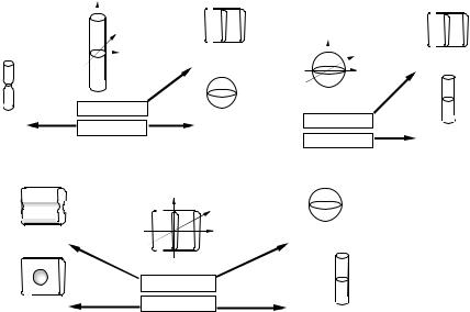
Figure 10.2: Schematic diagrams of measures of similarity to local structures. The roles of weight functions in representing the basic conditions of a local structure are shown. (a) Line measure. The structure becomes sheet-like and the
weight function ψ approaches zero with deviation from the condition λ3 λ2,
blob-like and the weight function ω approaches zero with transition from the
condition λ2 λ1 0 to λ2 λ1 0, and stenosis-like and the weight function
ω approaches zero with transition from the condition λ2 λ1 0 to λ1 # 0.
(b) Blob measure. The structure becomes sheet-like with deviation from the
condition λ3 λ2, and line-like with deviation from the condition λ2 λ1. (c)
Sheet measure. The structure becomes blob-like, groove-like, line-like, or pit-
like with transition from λ3 λ1 0 to λ3 λ1 0, λ3 λ1 0 to λ1 # 0,
λ3 λ2 0 to λ3 λ2 0, or λ3 λ2 0 to λ2 # 0, respectively. ( c 2004 IEEE)
The specific shape given in Eq. (10.3) representing the condition λt λs
(where t = 3 and s = 2 for the line case) is based on the need to generalize the
two line measures λmin23 and λg−mean23 [3]: |
|
|
|
|
|||||||
λmin23 = |
min( |
− |
λ2, |
− |
λ3) |
= − |
λ2 |
λ2 < 0 and |
λ |
3 |
< 0 |
0 |
|
|
|
otherwise. |
|
(10.5) |
|||||

538 |
Sato |
the derivative computation for the gradient vector and the Hessian matrix is combined with Gaussian convolution. By adjusting the standard deviation of Gaussian convolution, local structures with a specific range of widths can be enhanced. The Gaussian function is known as a unique distribution optimizing localization in both the spatial and frequency domains [20]. Thus, convolution operations can be applied within local support (due to spatial localization) with minimum aliasing errors (due to frequency localization).
We denote the local structure filtering for a volume blurred by Gaussian convolution with a standard deviation σ f as
Sξ { f ; σ f }, |
(10.11) |
where ξ {sheet, line, blob}. The filter responses decrease as σ f in the Gaussian convolution increases unless appropriate normalization is performed [21–23]. In order to determine the normalization factor, we consider a Gaussian-shaped model of sheet, line, and blob with variable scales.
Sheet, line, and blob structures with variable widths are modeled as
" |
|
|
= |
|
− |
2σr2 |
|
|
|
|
|
|
sheet (x ; σr ) |
|
exp |
|
x2 |
|
, |
|
|
(10.12) |
|||
|
|
|
|
|
|
|||||||
" |
|
= |
|
− |
2σr2 |
|
|
|
|
|
||
line(x ; σr ) |
|
exp |
|
x2 |
+ y2 |
, |
|
(10.13) |
||||
|
|
|
|
|
||||||||
and |
= |
|
− |
|
2σr2 |
|
|
|
|
|
||
" |
|
|
+ z2 |
|
|
|||||||
blob(x ; σr ) |
|
exp |
|
x2 |
+ y2 |
|
, |
(10.14) |
||||
|
|
|
|
|
|
|||||||
respectively, where σr controls the width of the structures.
We determine the normalization factor so that Sξ { ξ (x" ; σr ); σ f } satisfies the
following condition: |
|
|
|
|
||
S { |
ξ (0;" σr ); σ f |
} |
is constant, irrespective of σ f , where 0" |
= |
|
|
maxσr |
ξ |
|
|
(0, 0, 0). |
||
The above condition can be satisfied when the Gaussian second derivatives
are computed by multiplying by σ 2 as the normalization factor. That is, the |
||
f |
|
|
normalized Gaussian derivatives are given by |
f (x") |
|
fxp yq zr (x" ; σ f ) = 9σ 2f · ∂ xp∂ yq ∂ zr Gauss(x" ; σ f ): |
(10.15) |
|
∂2 |
|
|
where p, q, and r are non-negative integer values satisfying p + q + r = 2, and
Gauss(x" ; σ ) is an isotropic 3D Gaussian function with a standard deviation σ
√
given by ( 2π σ )−1 exp(−|x"|2/(2σ 2)) (see the Questions section at the end of

540 |
Sato |
of the line filter can be adjusted and widened using multiscale integration of filter responses given by
Mline{ f ; σ1, s, n} = |
max |
; |
σi}, |
(10.16) |
1 i n Sline{ f |
|
|
||
|
≤ ≤ |
|
|
|
where σi = si−1σ1, in which σ1 is the smallest scale, s is a scale factor, and n is the
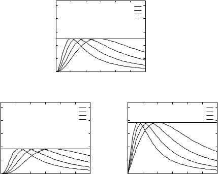
number of scales [7]. The width response curve of multiscale integration using
the four scales consists of the maximum values among the four single-scale
width response curves, and gives nearly uniform responses in the width range
√
between σr = σ1 and σr = σ4 when s = 2 (Fig. 10.3(a)). While the width
response curve can be perfectly uniform if continuous variation values are used for σ f , the deviation from the continuous case is less than 3% using discrete
|
|
|
|
|
|
|
|
|
|
|
values for σ f with s |
= |
√2 [7]. Similarly, in the cases of |
S |
|
{ |
2 |
} |
and |
||
|
|
sheet |
|
sheet (0", σr ); σ f |
|
|||||
S { " } ≈
blob blob(0, σr ); σ f , the maximum of the normalized response is (√3)3 ( 0.385)
|
|
σ f |
|
|
2 |
|
3 5 |
|
3 |
|
||
when |
σr = |
√ |
|
|
(Fig. 10.3(b)), |
and |
3 |
( |
5 ) |
(≈ 0.186) when σr = |
2 |
σ f |
2 |
|
|||||||||||
(Fig. 10.3(c)), respectively (see the |
Question section at the end of this chapter |
|||||||||||
|
|
|
|
|
|
|
||||||
for the derivation). For the second-order cases, the width response curve can be adjusted and widened using the multiscale integration method given by
Mξ { f ; σ1, s, n} = |
max |
{ f |
; |
σi}, |
(10.17) |
1 i n Sξ2 |
|
||||
|
≤ ≤ |
|
|
|
|
where ξ {sheet, line, blob}.
10.2.3 Implementation Issues
10.2.3.1 Sinc Interpolation Without Gibbs Ringing
Our 3-D local structure filtering methods described above assume that volume data with isotropic voxels are used as input data. However, voxels in medical volume data are usually anisotropic since they generally have lower resolution along the third direction, i.e., the direction orthogonal to the slice plane, than within slices. Rotational invariant feature extraction becomes more intuitive in a space where the sample distances are uniform. That is, structures of a particular size can be detected on the same scale independent of the direction when the signal sampling is isotropic. We therefore introduce a preprocessing procedure for 3-D local structure filtering in which we perform interpolation to make each voxel isotropic. Linear and spline-based interpolation methods are often used, but blurring is inherently involved in these approaches. Because, as noted above,
Hessian-Based Multiscale Enhancement and Segmentation |
541 |
the original volume data is inherently blurrier in the third direction, further degradation of the data in that direction should be avoided. For this reason, we opted to employ sinc interpolation so as not to introduce any additional blurring. After Gaussian-shaped slopes are added at the beginning and end of each profile in the third direction to avoid unwanted Gibbs ringing, sinc interpolation is performed by zero-filled expansion in the frequency domain [24, 25].
The method for sinc interpolation without Gibbs ringing is described below. The sinc interpolation along the third (z-axis) direction is performed by zero-filled expansion in the frequency domain. Let f (i) (i = 0, 1, . . . , n − 1) be the profile in the third direction. In the discrete Fourier transform of f (i), f (i) should be regarded as cyclic and then f (n − 1) and f (0) are essentially adjacent. Unwanted Gibbs ringing occurs in the interpolated profile due to the discontinuity between f (n − 1) and f (0). Thus, Gaussian-shaped slopes are added at the beginning and end of f (i) to avoid the occurrence of unwanted ringing before the sinc interpolation. Let f (i) (i = −3 · σ, . . . , 0, 1, . . . , n − 1, n, . . . , 3 · σ + n)
be the modified profile, which is given by |
|
|
|
|
|
|
|
|
||||||||||||||
|
|
|
exp(− |
i2 |
|
) |
· |
f (0) |
|
|
|
i |
−3 · σ, . . . , 0 |
|
|
|
||||||
|
|
|
2σ |
2 |
|
|
|
|
|
|
||||||||||||
f (i) |
= |
f (i) |
|
|
|
|
|
|
|
|
|
|
i = |
0, . . . , n |
− |
1 |
(10.18) |
|||||
|
|
|
|
(i n 1)2 |
) |
|
( |
|
1) |
= |
|
3 |
|
|
|
|
||||||
|
|
exp( |
− |
− + |
|
· f |
n − |
i = n, . . . , |
· σ |
|
|
|
||||||||||
|
|
|
|
|
2σ 2 |
|
|
|
|
|
|
|
(3 |
|||||||||
where the variation is sufficiently smooth everywhere, including between |
|
|||||||||||||||||||||
|
|
|
|
|
|
|
|
|
|
|
|
|
|
|
|
|
|
|
|
|
f |
· |
|
|
|
|
|
|
|
|
|
|
|
|
|
|
|
|
|
|
|
|
|
||
σ + n) and f (−3 · σ ). The discrete Fourier transform of f (i) is performed (we used σ = 4). After the sinc interpolation of f (i), the added Gaussian-shaped slopes are removed.
10.2.3.2 Computation of Gaussian Derivatives and Eigenvalues
The computation of the Gaussian derivatives in the Hessian matrix and the gradient vector (needed in the later chapters) can be implemented using three separate convolutions with 1-D kernels as represented by
fxp yq zr (x" ; σ f ) = |
9 |
∂ xp∂∂yq ∂ zr Gauss(x" ; σ f ): f (x") |
|
||||||
|
|
|
2 |
|
|
|
|
|
|
= dxp Gauss(x ; σ f ) |
9dyq Gauss(y ; σ f ) |
|
|||||||
|
|
dp |
|
|
dq |
|
|
||
|
|
|
9dzr Gauss(z ; σ f ) f (x"):: |
(10.19) |
|||||
|
|
|
|
dr |
|
|
|
|
|