

Kluwer - Handbook of Biomedical Image Analysis Vol
.2.pdf462 |
Suri et al. |
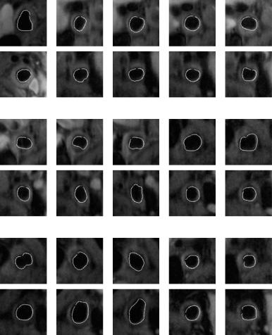
Figure 9.5: Abnormal ground truth overlays. The top row in each row pair is the left carotid artery overlayed with the ground truth tracing of the inner lumen wall, and the bottom row is the corresponding image of the right carotid artery. Some lumens have a circular shape, while others have an elliptical shape.
9.2.1 Ground Truth Tracing and Data Collection
Figures 9.5–9.9 show abnormal images of the left and right carotid arteries overlayed with the ground truth tracing. In each pair of rows, the top row is the left carotid arteries and the bottom row is the right carotid arteries. The ground truth tracing is the boundary of the inner lumen wall. Figure 9.9 shows the normal images of the same left and right carotid arteries. The normal images show
Lumen Identification, Detection, and Quantification in MR Plaque Volumes |
463 |
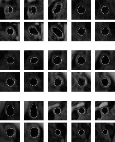
Figure 9.6: Abnormal ground truth overlays. The top row in each row pair is the left carotid artery overlayed with the ground truth tracing of the inner lumen wall, and the bottom row is the corresponding image of the right carotid artery. Some lumens have a circular shape, while others have an elliptical shape.
lumens that are more circular than those of the abnormal images, and there is no constriction of the arteries. Ground truth tracing was done using the MATLAB program MRI GUI ver 1.2. For each lumen boundary the image was zoomed in and points were plotted by the user around the inner wall boundary. The points were spline-fitted to 20 points.
The imaging parameters (TR/TE/TI/NEX/thickness/FOV/ETL) are as following: T1W:1R-R/7.1 ms/500 ms/2/3 mm/12–14 cm/21; PDW: 2R-R/7.1 ms/600 ms/
464 |
Suri et al. |
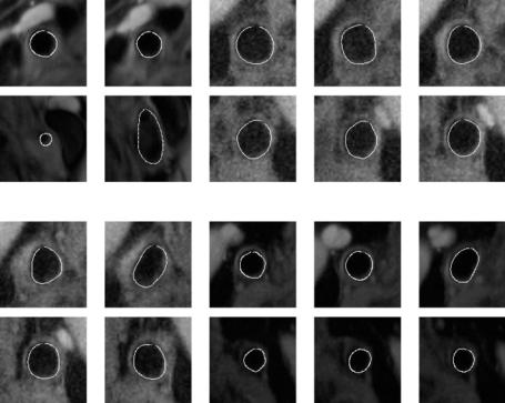
Figure 9.7: Abnormal ground truth overlays. The top row in each row pair is the left carotid artery overlayed with the ground truth tracing of the inner lumen wall, and the bottom row is the corresponding image of the right carotid artery. Some lumens have a circular shape, while others have an elliptical shape.
2/3 mm/12–14 cm/31; T2W: 2R-R/68 ms/600 ms/2/3 mm/12–14 cm/31. Matrix for all images were 256 × 192. Voxel size was 0.5 × 0.5 × 3 mm3. For bright blood 3D TOF images: TR/TE/flip angle/thickness/FOV = 20 ms/3.4 ms/25/2.0 mm/18. Zero-filled Fourier transform was used to create voxels of 0.35 × 0.35 × 1 mm3 for 3-D TOF imaging. The factors which affect MR plaque quality are (a) random patient motion, including (b) obese patients who may have deeper carotid arteries, (c) incomplete flow suppression, and (d) artery wall pulsation.
Lumen Identification, Detection, and Quantification in MR Plaque Volumes |
465 |
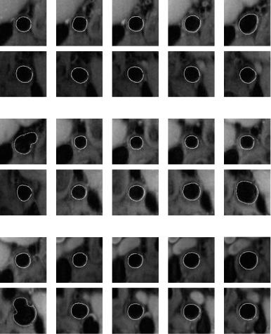
Figure 9.8: Abnormal ground truth overlays. The top row in each row pair is the left carotid artery overlayed with the ground truth tracing of the inner lumen wall, and the bottom row is the corresponding image of the right carotid artery. Some lumens have a circular shape, while others have an elliptical shape.
9.3Three Pixel Classification Algorithms: MRF, FCM, and GSM
9.3.1 Markovian-Based Segmentation Method
The algorithm consisted of running the pixel classification approach using Markov random field with mean field (see Zhang [149]). Here, the image segmentation was posed as a classification problem where each pixel is assigned to one of K image classes. Suppose the input image was y = {yi, j , (i, j) L}, where yi, j is a pixel, i.e., a 3-D vector, and L was a square lattice. Denote the segmentation as z = {zi, j , (i, j) L}. Here, zi, j is a binary indicator vector of dimension K , with only one component being 1 and the others being 0. For
Lumen Identification, Detection, and Quantification in MR Plaque Volumes |
467 |
where and were model parameters. In this work, we assume that the pixels in y are conditionally independent given z, i.e.,
log p(y | z, ) = log p(yi, j | zi, j , ). (9.2)
i, j
Furthermore, we assume that conditioned on zi, j , the pixel yi, j has a multivariate Gaussian density, i.e., for k = 1, 2, . . . , K,
|
|
|
|
|
e− 21 (yi, j |
− |
mk)T C−1 |
(yi, j |
− |
mk) |
|
|
p(y |
z |
e |
, ) |
= |
|
k |
|
|
, |
(9.3) |
||
|
(2π )3/2|Ck|1/2 |
|
|
|||||||||
i, j | |
i, j = |
k |
|
|
|
|
|
|
||||
where ek is a K -dimensional binary indicator vector with the kth component being 1. From this, = {mk, Ck}kK=1 contained the mean vectors and covariance matrices for the K image classes. For z, we have adopted an MRF model with a Gibbs’ distribution [149]:
p(z |
| |
) |
= |
1 |
e−βE(z), |
(9.4) |
|||
|
|||||||||
|
|
|
|
|
Z |
|
|||
where |
|
|
|
|
|
|
|
|
|
|
1 |
|
|
|
|||||
E(z) = |
|
|
|
|
|
|
|
1 − 2zit, j zk,l |
(9.5) |
2 |
|
|
|
|
|
||||
|
|
|
|
i, j (k,l) Ni, j |
|
||||
is the energy function which decreased (causing p(z | ) to increase) when neighboring pixels were classified into the same class (the set of the neighbors of (i, j) is denoted as Ni, j ).
Since was generally not sensitive to particular images, it was set manually here. , on the other hand, was directly dependent on the input image and hence had to be estimated during the segmentation process. In this work, as it in [149], this was achieved by using the EM algorithm [177], which amounts to iterating between the following two steps:
1. E step: Compute
ˆ ( p) |
ˆ |
( p) |
. |
Q( | |
) = log p(y | z, ) + log p(z | ) | y, |
|
2. M step: Update parameter estimate
( p+1) = arg max Q( | ( p)).
Here · represents the expectation, or mean, and the superscript p denotes the pth iteration. This translated into the following formulas for updating the
468 |
|
|
|
|
|
|
|
|
|
|
|
|
|
|
Suri et al. |
parameter estimates: |
|
|
|
|
|
|
|
|
|
|
|
|
|
|
|
zi(,pj) |
8 |
= zi, j |
zi, j f (zi, j ) |
|
|
|
|
|
|
|
(9.6) |
||||
7 |
= |
|
|
( p) |
|
|
|
|
|
|
|
|
|
|
|
|
|
i,7j zi,8j |
|
|
|
|
|
|
|
|
|||||
mˆ ( p+1) |
|
i, j |
zi, jk |
yi, j |
, |
|
|
|
|
|
|
|
|
||
k |
|
|
|
z7( p) |
k y8 i, j |
|
mˆ ( p+1) yi, j |
mˆ ( p+1) T |
|
|
|||||
ˆ ( p 1) |
= |
7 |
i, jk |
82 |
|
− |
|
i, j zi, j32 |
− k |
3 |
|
|
|||
|
i, j |
|
|
|
k |
|
|
|
|
||||||
Ck + |
|
|
|
|
|
|
|
|
|
|
|
|
|
, |
(9.7) |
|
|
|
|
|
|
|
|
|
7 |
k 8 |
|
|
|
|
|
where k = 1, 2, . . . , K, zi, jk is the kth component of zi, j , and f (zi, j ) a “mean field” probability distribution (see Zhang [149]).
These formulas, in addition to providing the estimate of , also produced a
segmentation. Specifically, at each iteration, z( p) was interpreted as the prob-
i, jk
ability that yi, j was assigned to class k. Hence, after a sufficient number of iterations, we can obtain the segmentation z for each (i, j) L by
zi, j = ek0 if k0 = arg max1≤k≤K zi, jk . |
(9.8) |
In this way, the EM procedure described above generated the segmentation as a by-product, and therefore provided an alternative to the MAP solution of Eq. (9.1) For those interested in the application of MRF in medical imaging, see Kapur [150], who recently developed a brain segmentation technique which was an extension to the EM work of Wells et al. [174] by adding the Gibbs’ model to the spatial structure of the tissues in conjunction with a mean-field (MF) solution technique, called Markov random field (MRF) technique (for details on MRF, see Li [151] and Geman and Geman [179]). Thus the technique was named expectation maximization–mean field (EM–MF) technique. By Gibbs’ modeling of the homogeneity of the tissue, resistance to thermal noise in the images was obtained. The image data and intensity correction were coupled by an external field to an Isinglike tissue model, and the MF equations were used to obtain posterior estimates of tissue probabilities. This method was more general to the EM-based method and is computationally simple and an inexpensive relaxation-like update. For other work in the area of MRF for brain segmentation see Held et al. [152].
Pros and Cons of MRF with Scale Space. The major advantages of MRFbased classification is (1) addition of Gibbs’ Model: Kapur et al. model the a priori assumptions about the hidden variables as a Gibbs’ random field. Thus the prior probability is modeled using the following physics-based analogous Gibbs’
Lumen Identification, Detection, and Quantification in MR Plaque Volumes |
469 |
||||||
1 |
1 |
|
E( f ) |
|
|
||
equation: P( f ) = |
|
exp(− |
|
)E( f )), where Z = f exp( − T |
) and P( f ) is the |
||
Z |
κ T |
||||||
probability of the configuration |
f , T is the temperature of the system, κ is the |
||||||
Boltzmann constant, and Z is the normalizing constant. The major disadvantages of MRF-based classification include the following: (1) The computation time would be large if the number of classes is large. In such cases, one needs to use the multiresolution techniques to speed up the computation. (2) The positions of the initial clusters are critical in solving the MRF model for the convergence. Here, the initial cluster was computed using K -means algorithm which was a good starting point. However, a more robust method is desirable.
9.3.1.1 Implementation of MRF System
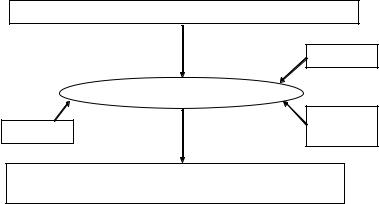
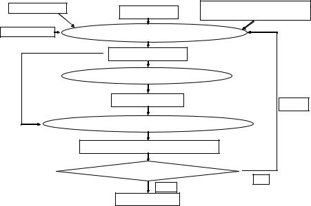
Figure 9.10 shows the main MRF classification system implementation. Input is a perturbed gray scale image with left and right lumens. The number of classes, the initial mean, and the error threshold are inputs given to the system. The result is a classified image with multiple class regions in it, including multiple classes in the lumen region. Figure 9.11 shows the MRF system in more detail. Given the initial center, the number of classes K , the Markov parameters of mean, variance, and covariance, and the perturbed image, the current cluster center is calculated. Using the EM algorithm, new parameters are solved and new cluster
|
Gray Scale Perturbed Image with Multiple Lumens |
|
K (classes) |
|
Classification Process |
|
Error |
Initial Mean |
Threshold |
Classified Image with Multiple Lumens and Each Lumen Having
Multiple Class Regions
Figure 9.10: Markov random fields (MRF) classification process. Input is a gray scale perturbed image with left and right lumens. The number of classes, the initial mean, and the error threshold are inputs given to the system. The result is a classified image with multiple class regions in it.
470 |
|
Suri et al. |
|
# of Classes (K) |
Perturbed Image |
Markov Parameters: Mean, |
|
Variance, Covariance |
|||
|
|||
|
|
||
Initial Center |
Current Cluster Center |
|
|
|
Current Cluster Center |
|
EM Algorithm for Solving Φ
New Cluster Centers
Update
Compare Error Between Two Cluster Centers
Error Difference Between Cluster Centers
Is Error less than Threshold?
NO
YES
Segmented Image
Figure 9.11: The Markov random fields (MRF) segmentation system. Given the initial center, the number of classes K , the Markov parameters of mean, variance, and covariance, and the perturbed image, the current cluster center is calculated. Using the expectation-maximization (EM) algorithm, new parameters are solved and new cluster centers are computed. The error between the previous cluster center and the recently calculated cluster center are compared, and the process is repeated if the error is not less than the error threshold. After the iterative process is finished, the output is a segmented image.
centers are computed. The error between the previous cluster center and the recently calculated cluster center are compared, and the process is repeated if the error is not less than the error threshold. After the iterative process is finished, the output is a segmented image.
9.3.2 Fuzzy-Based Segmentation Method
In this step, we classified each pixel. Usually, the classification algorithm expects one to know how many classes (roughly) the image would have. The number of classes in the image would be the same as the number of tissue types. A pixel could belong to more than one class, and therefore we used the fuzzy membership function to associate with each pixel in the image. There are several
