Kluwer - Handbook of Biomedical Image Analysis Vol
.2.pdf342 |
Walter and Klein |
it must be connected to a dilated version of the main branches of the vascular tree:
v(x) = |
tmin |
if |
x V |
|
|
|
tmax |
if |
x |
V |
|
|
|
|
|
|
|
l1 = R fl δsBv fl |
with s = 5 |
(7.21) |
|||
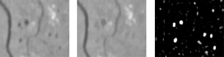
It is recommended not to use the complete vascular tree V , but only the main branches that can be extracted easily by applying a stronger contrast criterion in the algorithm presented in section 7.5.1.
The effect of this filtering is shown in Fig. 7.21: The atrophy present in the image (a) is removed in (b), the optic disk stays nearly entirely unchanged by the reconstruction. Using the methods presented in [14, 17, 18], the localization algorithm would have failed in this case.
Now, we can assume that the optic disk belongs to the brightest elements of the image, and the application of an area threshold should give a part of the optic disk:
L1 = T[α,tmax ](l1) with α such that #L1 ≥ K |
(7.22) |
L1 normally contains more than one connected component: A part of the optic disk, some noise, and eventually other bright features connected to the vascular tree. The latter ones are normally exudates of small size. Hence, it is sufficient to choose the connected component with the largest surface to obtain a part of the optic disk:
L C(L1) with A C(L1) : #L ≥ # A |
(7.23) |
The center of the (only) connected component of L can be seen as the approximative center c of the optic disk and is used for the detection of the contours described in the following paragraph.
Detection of the contours: The contours of the optic disk appear under the best contrast in the red channel fr of the color image. Unfortunately, the red channel is sometimes saturated and cannot be used. In this case, we propose to work on the luminance channel fl. The first step is to determine if the red channel is saturated or not. Let c be the approximative center determined in the localization step of the algorithm, fr a subimage of the red channel centered in c, and tmax( fr) the maximal gray-level value within this subimage. We define the
Analysis of Color Fundus Photos and Its Application to Diabetic Retinopathy |
343 |
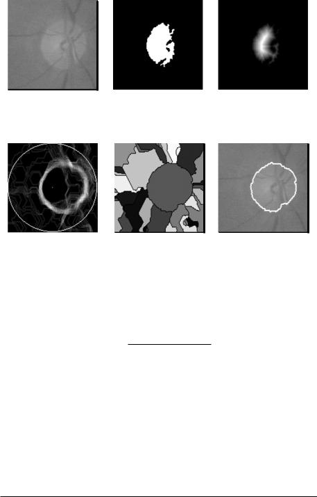
(a) The luminance chan- |
(b) The biggest particle |
(c) The distance func- |
nel |
of the threshed image |
tion of the particle |
(d) The gradient image with the superposed marker
(e) The result of the |
(f) The segmentation |
watershed algorithm |
result |
Figure 7.22: The steps of the algorithm for the detection of the contours.
gray-level saturation Sα 3:
Sα = |
#T[tmax ( fr )−α,tmax ( fr )]( fr) |
(7.24) |
#T[0,tmax ( fr )]( fr) |
This measure determines the percentage of pixels in the subimage whose gray level is larger than tmax( fr) − α. If this percentage is too high, the channel is saturated and does not contain any exploitable information. We use the red channel, if for α = 30, Sα < 0.5 (this has been found experimentally), if not, the luminance channel is used. We call the used channel fc in the following.
For finding the contours of the optic disk, we shall make use of the watershed transformation applied to the gradient image of a filtered version of the channel fc (see also Fig. 7.22).
3 The gray-level saturation Sα should not be confounded with the color saturation.
344 |
Walter and Klein |
First, we attenuate the noise in the image using a Gaussian filter G (type and parameters of the filter are not crucial, we used a 9 × 9 filter with σ = 4). Then, the vessels interrupting the circular shape of the optic disk are filled using a morphological closing:
p1 = φ(s1 B)(G fc) |
(7.25) |
with s1 such that the largest vessels are filled (as explained in the previous section). In order to remove irregularities within the papillary regions that may also produce a high-gradient value, we apply an opening by reconstruction:
p2 = Rp1 (ε(s2 B)( p1)) |
(7.26) |
s2 |
= 15 has been found to be |
a good value for 640 × 480 images. This is |
|
a |
big opening, but thanks to the reconstruction, the contours of p1 are |
||
preserved. |
|
|
|
|
Then, the morphological gradient is calculated: |
|
|
|
ρp2 |
= δ(B) p2 − ε(B) p2 |
(7.27) |
Calculating the watershed transformation of this gradient would lead to a strongly oversegmented result. Once again, we have to find a marker and impose it (see section 7.3). With only one source within the optic disk, the algorithm gives exactly one catchment basin which—if the filtering process has been efficient— coincides exactly with the optic disk. We use the approximated center c as “inner marker.” As external marker, we use a circle centered in c with a diameter larger than two times the largest possible diameter of the papilla (factor 2 for the case that the approximation was bad and the approximation of the center c lies on the border of the optic disk).
m(x) |
= |
ρp2 |
if |
x {c} Cercle(c) |
(7.28) |
|
tmax |
if |
x {c} Cercle(c) |
|
|
|
|
|
With this marker, we can now calculate the watershed transformation:
Pf in = C Vi |
2Rρp2 (m)3 |
with c C Vi |
(7.29) |
7.5.2.5 Results
The algorithm has been tested on 60 color fundus photographs (640 × 480) taken with a Sony color video 3CCD camera on a Topcon TRC 50 IA
Analysis of Color Fundus Photos and Its Application to Diabetic Retinopathy |
345 |
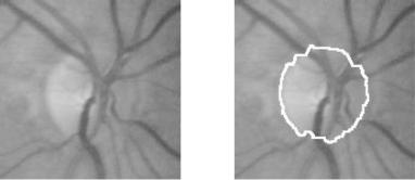
(a) The optic disk in a color |
(b) Segmentation result |
image
Figure 7.23: Detection of the optic disk.
retinograph. These images have not been used for the development of the algorithm.
The optic disk has been localized correctly in 57 of these 60 images. In 3 of these 60 images, there were very large accumulations of exudates which inhibited a correct localization of the optic disk. The accuracy of the detection of the contours has been assessed qualitatively by a human grader; there were 48 images, for which the segmentation result was satisfying, with no or few pixels missed or falsely detected (e.g. see Fig. 7.23). In eight images, there were some parts missing due to very poor contrast of the original images, but the result contained still more than 75% of the optic disk. In one image, the result was not satisfying, once again due to low contrast: Indeed the contour was hardly visible, even for a human.
7.6The Detection of Pathologies in Color Fundus Images
Pathology detection is certainly the most important part of analysis of retinal images. In diabetic retinopathy, there are three types of lesions indicating different stages of the disease that can be detected using color fundus images: microaneurysms, exudates, and hemorrhages. In this section, we present automatic algorithms for the detection of microaneurysms and exudates. An algorithm for the detection of hemorrhages can be found in [9].


348 |
Walter and Klein |
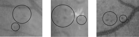
(a) A detail of a fundus |
(b) Detail of the prefiltered |
image containing microa- |
image |
neurysms |
|
Figure 7.26: Prefiltering step.
The detection of dark isolated details by means of the diameter closing: The next step is to find the “candidates,” i.e., all features that may possibly correspond to microaneurysms. Microaneurysms are characterized by their diameter; in the green channel of a color image, they correspond to dark details—“holes”—with a maximal diameter of λ (with λ depending on the image resolution).
As in the top-hat transformation used for vessel detection in section 7.5.1, the main idea is to first construct a closing φ that removes the details from the image and then calculate the difference to the original image. However, a morphological closing cannot be used in our case because it fills not only the holes but also the ditches (vessels). One possibility to fill only the holes without filling the ditches is to determine the infimum of openings with linear structuring elements in different directions, because they do fit into the vessels in at least one direction. However, this is only an approximative solution of the problem; a tortuous line for example will be closed as well. We will now present the diameter closing φλ◦ which removes all dark details of a diameter smaller than λ.
First, we define the diameter α of a connected set X as its maximal extension, i.e. the maximal distance between two points of the set:
5
α (X) = |
d(x, y) |
(7.31) |
x,y X
with d(x, y) the distance between two points x and y. For simplicity, we use the block distance: If x = (x1, x2), y = (y1, y2) Z2 are two points and x1, x2 and y1, y2 their coordinates, respectively, the block distance can be written as d(x, y) = |x1 − y1| |x2 − y2|.

Analysis of Color Fundus Photos and Its Application to Diabetic Retinopathy |
349 |
(a) A binary image |
(b) The result of a diameter opening |
Figure 7.27: The diameter opening of a binary image: all connected components with a diameter inferior to 15 pixels are removed.
With this definition of the diameter of a set, we can define a trivial opening.
Let X be an arbitrary binary image and Xi its connected components, i.e. X =
0
Xi and Xi ∩ X j for i = j. The diameter opening is the union of all connected components Xi with a diameter greater or equal to λ (see Fig. 7.27):
|
◦ |
(X) |
α("i ≥ |
X |
|
(7.32) |
γ |
= |
i |
||||
|
λ |
|
|
|
||
|
|
|
X ) |
λ |
|
|
As the applied criterion α(Xi) ≥ λ is increasing, i.e., X Y implies that if X fulfills the criterion, Y also does, the operation γλ◦(X) is an opening.
It can be shown that the diameter opening is the supremum of all open-
ings with structuring elements with a |
diameter greater than |
or equal to |
||||
λ [8]: |
|
|
α("≥ |
|
|
|
|
◦ |
(X) |
γ B(X) |
(7.33) |
||
γ |
= |
|
||||
|
λ |
|
|
|
|
|
|
|
|
B) |
|
λ |
|
It is, therefore, a generalization of the approximative method proposed in [16] used by the majority of authors, where only linear structuring elements fulfilling the criterion are used.
The diameter closing removes all holes Xic (connected components of the background Xc) with a diameter inferior λ. Furthermore, it can be written as the infimum of all morphological closings with structuring elements whose diameter

350 |
Walter and Klein |
|
|
|
x |
flooding level s |
|
|
|
C |
X |
− |
(f) |
x |
|
s |
|
|
|
|
Xs− (f) |
Figure 7.28: The flooding of an image f at level s. |
|||
is equal or superior to λ:
|
φλ◦(X) (x) = X |
|
c |
Xic |
||
2 |
3 |
|
α("i |
|
||
|
B |
|||||
|
α(6≥ |
|
|
X )<λ |
|
|
|
φ |
|
(7.34) |
|||
|
= |
|
|
|||
|
B) |
|
λ |
|
|
|
We have now defined the diameter opening and closing for the binary case. In order to pass from binary to gray-level images, we can apply the binary operator to all level sets (the results of threshold operations for all gray levels t T ). Let
Cx(X) be the connected opening, i.e., the connected component of X containing x if x X and the empty set if x / X. Furthermore, let Xt+( f ) be the section of f at level t, i.e., the set of all pixels for which f (x) ≥ t and Xt−( f ) the section of the background (the “lakes,” see Fig. 7.28):
X+( f ) |
= |
T |
|
( f ) |
= { |
x |
|
E |
| |
f (x) |
≥ |
t |
} |
(7.35) |
||
t |
[t,tmax ] |
|
|
|
|
|
|
|
||||||||
X−( f ) |
= |
T |
( f ) |
= { |
x |
|
E |
| |
f (x) |
≤ |
t |
} |
|
|||
t |
[tmin ,t] |
|
|
|
|
|
|
|
|
|||||||
Then, the gray scale diameter opening and closing can be defined respectively:
φ◦ |
|
|
# |
|
|
|
|
|
|
|
x |
|
2 |
− |
|
|
3 |
|
|
$ |
|||
γ |
◦ |
( f ) |
= |
sup |
s |
≤ |
f (x) |
|
| |
α |
C |
x |
X+ |
( f ) |
≥ |
λ |
|||||||
|
λ |
|
# |
|
|
|
| |
|
|
|
|
|
s |
|
|
$ |
|||||||
|
λ |
( f ) |
= |
s |
≥ |
f (x) |
|
|
|
2 |
X |
s |
|
|
3 ≥ |
λ |
|||||||
|
|
|
inf |
|
|
|
|
α C |
|
|
|
|
( f ) |
|
(7.36) |
||||||||
Of course, Eq. (7.36) cannot be used for implementation of this algorithm because it would be highly inefficient. Instead of calculating the diameter opening