Kluwer - Handbook of Biomedical Image Analysis Vol

contour is more likely to be a boundary point, its a posteriori probability with label p and q will be quite similar. It then leads to the value of r(s) being closer to 1 and makes point s more reliable. Therefore, in the control point searching process, we use maximum reliability as a criterion, which can be expressed as

The above criterion can be applied directly to the boundary points obtained with the QHCF algorithm because of the location and shape accuracy of the found object region. A further advantage of this accuracy is the solid foundation from which to do further work. This foundation is similar to the manual outline provided by the human operator for the traditional Snake algorithm. Consequently, use of the MRF-based segmentation result and the MAP criterion allows for an automatic initialization process that is relatively free of traps due to noise and spurious edges and has consistent reproducibility.

Step 2 addresses the selection problem of section number M and size of each section. Image quality and confidence of the contour points are determining factors in finding the solutions. For example, in our carotid lumen segmentation of MR images shown in Fig. 8.18, typical images generally needed 3–6 sections for contour tracking, while low-quality images required 8–10 splitting sections to track the whole blood vessel boundary. Object boundary corruption by noise results in more splits in the attempt to attain higher accuracy. The size of the object also is an important factor. Most of our studies contain objects sequestered within a square the size of 128 by 128 pixels. Division of the contour is accomplished by equal-length splitting. A more dynamic approach can be used in the case of a contour with noisier pixels resulting in more control points for ACM. The resulting curve will be noise-resistant and reliable. In addition, processing speed will be increased.

Step 1 is the most flexible and application-dependent of the three steps. It may also be totally eliminated in cases that target regions are already known. However, in most situations lack of advance knowledge of the exact location and spurious knowledge of the object’s properties can be referenced as an additional constraint during the segmentation process. When this occurs an identification process can be designed based on the QHCF segmented regions to extract the boundary of the region-of-interest, which can then be used in further contour fine-tuning. An example is the lumen segmentation in a sequence of MR images.

P1

P0

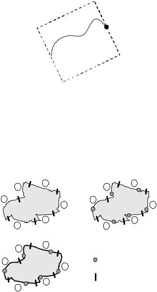
Figure 8.8: Illustration of the dynamic searching range frame.

involve a lot calculation to control its boundary. For simplicity and generality, we chose the square region to limit searching range. Another benefit of this restriction is that it can work as a control of the overall object shape and prevent the occurrence of “wild divergence” distorted by noise.

The procedure of region boundary splitting, control point searching, and curve fine-tuning is illustrated in Fig. 8.9.

- section separator

5

6

(c)

Figure 8.9: Illustration of the procedure used to apply the MRF-based active contour model on object boundary tracking. (a) The QHCF segmented region with the boundary divided into six sections. (b) In each section, a control point is searched based on maximum reliability criterion. (c) The final fine-tuned contour is found by linking the curves between each two adjacent control points, which are searched with minimal path approach.

8.3.4 Simulation Results

In this section, we present some experimental results of the proposed framework.

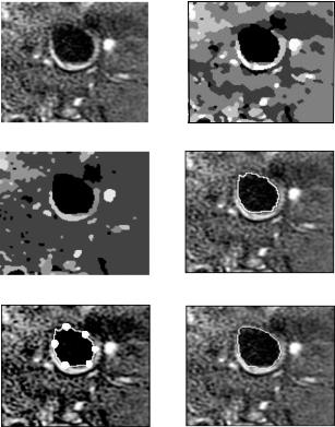
8.3.4.1 Segmentation of Single Image

First, a typical carotid MR image is shown in Fig. 8.10(a). Because of the noise or artifacts during imaging process, the intensity of lumen area is not uniform and there are some isolated bright spots inside. The QHCF algorithm was applied to this image and segmented it into many regions as shown in Fig. 8.10(c). From the result, we can see that the lumen segmentation is not affected by those bright spots inside the lumen area and most of the noise in the background have been suppressed. This is better than the result segmented with adaptive ICM algorithm shown in Fig. 8.10(b). By tracking the boundary of lumen region based on purely QHCF segmented results, we obtained the contour points of target region as shown in Fig. 8.10(d). It is obvious that some sharp corners on the top-left part of the contour and the bottom part are also not very smooth; this conflicts with normal observation of lumen shape in anatomy. In the next step, this contour was split into six equal sections and we searched the control points (see Fig. 8.10(e)) with maximum reliability criterion. The MPA algorithm was then used to track the whole contour and the result is shown in Fig. 8.10(f). Compared with the contour in Figs. 8.10(d) and 8.10(f), the effect of smoothness constraint in MPA algorithm is demonstrated. The two rough parts in Fig. 8.10(c) have also been fine-tuned.

8.3.4.2Atherosclerotic Blood Vessel Tracking and Lumen Segmentation

Most existing active contour model based algorithms require the topology of the object to be known before the tracking action starts. Unfortunately, this requirement is difficult to be satisfied in some practical scenarios since the topography is often difficult to be predicted in advance. For example, in our study of carotid artery, the lumen bifurcates from one common carotid artery into internal and external carotid arteries at certain location along the image

Figure 8.10: An example of lumen segmentation with MRF-based active contour framework. (a) The original MR image. (b) Segmentation results with adaptive ICM. (c) Segmentation results with the QHCF algorithm. (d) Rough lumen contour based on the QHCF segmentation result. (e) The six selected control points for MPA model initialization. (f) The fine-tuned lumen contour achieved by applying the MPA algorithm. In comparing (d) and (f), it becomes clear that contour tracking under the proposed framework results in superior smoothness control than with the MRF-based solution.

sequence. It is normally impossible to know where this kind of topological transformation happens.

8.3.4.2.1 Lumen Region Identification. To address the problem of topographical changes, we integrated prior knowledge into the control points

searching procedure. The bulk of our work is represented by the second block in the processing diagram shown in Fig. 8.7.

First, we model the MR image with MRF model and segment each of them into many regions by applying the QHCF algorithm. Since the number of lumen region may vary due to the bifurcation of carotid artery along the image sequence, a lumen identification process is indispensable before further plaque analysis. For each image, the lumen identification is achieved by letting all the segmented regions through a knowledge-based decision tree and picking up lumen region(s) of interest. The decision criteria are obtained by analyzing the statistical distribution of lumen region features based on prior knowledge in the test dataset. In the atherosclerotic blood vessel study, the following features are regarded critical for lumen identification:

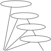
The basic structure of the decision tree is shown in Fig. 8.11. For criteria

CArea, CIntensity, and CCircularity, statistical analysis of training MR image data required the use of two standard deviations as the satisfactory scale to make sure most of the variation range can be covered. For CLocation, it reflects the maximum radius of lumen center may locate in current slice away from the center of lumen in the previous slice. To reduce the computation in the identification process, the most distinctive feature of the target region is always analyzed first so as to decrease the number of candidates in the following criteria checking. In our study, the sequence is arranged as CArea, CIntensity, CLocation, and

CCircularity.

From above identification procedure, it can be seen that the accuracy of the low-level region segmentation plays a very important role in the topography detection. This can be achieved by using the QHCF algorithm. For the lumen

CIntensity is

No Yes

CArea is

No Yes

CLocation is

No Yes

CCircularity is

No Yes

Figure 8.11: Diagram of the decision tree structure for lumen identification in MR image sequences.

identification step, however, if the choice of training dataset is sufficiently representative, those criteria will be fairly precise and hence make the decision result more stable. To further enhance the lumen tracking ability along image sequence, the location correlation of lumen regions between adjacent MR slices can be constrained by CLocation, which can further limit the searching range and therefore reduce computation.

8.3.4.2.2 Experiments and Discussion. In this study, 20 MR image sequences were tested with the proposed method. These images were scanned by a 1.5T SIGNA scanner (GE Medical Systems, 5.7 Echo Speed, custom made phased-array coils) in two imaging contrast weightings: T1-weighted (T1W) and 3D time-of-flight (3D TOF). Each mode produces 10 sequences with the bifurcation inside and 12 slices in each sequence.

It is well known that some feature characteristics appear altered by different modalities. The T1W sequence produces a lower intensity of the lumen signal. In 3D-TOF images, the intensity of the lumen is both higher and more uniform because of flow enhancement during imaging. For each contrast weighting, five sequences were selected for identification criteria estimation and the rest were used as testing data. Table 8.2 shows estimated criteria. The error rate is defined as the ratio between number of regions with error detection (misdetection or false alarm) and total number of lumen regions.

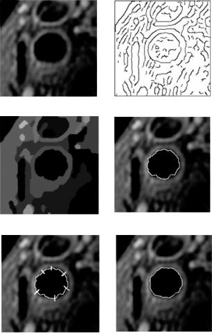
Figure 8.12: An example of the MRF-based active contour framework. (a) The original image of T1W MR image on carotid artery lumen. (b) Edge map by Canny edge detector. (c) Segmentation result of QHCF algorithm with Trc = 10, β1 =

400, β2 = 1000, Tmin = 20. (d) Lumen contour based on the QHCF algorithm.

(e) Six selected control points. (f) Fine-tuned contour by applying MPA.

segmentation and ACM models. In addition, it is also very flexible and can easily include prior knowledge from various applications. An example of blood vessel tracking and lumen segmentation in magnetic resonance image sequences is studied and the experimental results have demonstrated very satisfactory performance.

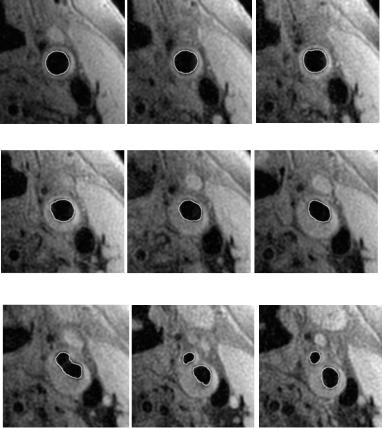
Figure 8.13: MR images of a human carotid artery from proximal common

(a) through the bifurcation that occurs between images (g) and (h) to the distal internal and external carotids (j). Tracked lumen boundaries are visualized as distinct lines separating the lumen from adjacent tissues. This series also illustrates the topology change tracking ability of the proposed framework from the single lumen of the common carotid to the two lumens of the bifurcation, internal, and external carotid arteries. The location of real bifurcation happens between image (g) and (h). The closed bright curves along lumen boundary are the tracked contours. These results also demonstrate the topology change handling ability of the proposed framework.