

Kluwer - Handbook of Biomedical Image Analysis Vol
.2.pdf502 |
Suri et al. |
9.6.1.1Lumen Area Computation by Triangle/Scan-Line Methods (A)
To determine the average area of the entire lumen from the ground truth boundaries, the area by triangles computation is used. The center point of the ROI is the user input, and is equivalent to the center of gravity (CG). The area of the enclosed region is obtained by summing the areas of the triangles formed by the CG and each pair of neighboring points on the boundary.
In the scan-line method, we count the number of pixels along the scan line which lies in the ROI. This process is done for all the lies which interest the ROI region. The entry and exit points are computed by finding the number of times the scan line interests the boundary yielding the odd or even number. If the intersection yields 1 then begin counting the pixels, and if the intersection yields 2, then stop counting pixels. This gives a total number of pixels along the line. The process stops when there are no more interesections. In a 384 × 512 image, the average area for the left and right lumen is 500 pixels squared.
9.6.1.2 Area of Lumen Core Class (B)
The select class package takes as one of its inputs the number of classes formed after the segmentation method. Using this as a size for an array of the different classes C0 through Cn, the program checks each pixel in the ROI and stores the number of times that each of the different pixel values occur. The program then sorts these class values by their frequency.
9.6.1.3Difference Computation (A − B) and Comparison with Threshold
Using the average ground truth contour area, a difference threshold, Td, is determined. We set Td = 75. If the difference between the average ground truth contour area and the number of pixels of C0 in the ROI is less than the difference threshold, then only C0 is selected. If the difference is greater than the difference threshold, then both C0 and C1 are selected, then they are merged and a binary image is made.
In the GSM, a select class package is not used, but a region growing method is used. The GSM usually merges the C0 and C1 classes, so the region growing captures both C0 and C1 classes.
Lumen Identification, Detection, and Quantification in MR Plaque Volumes |
503 |
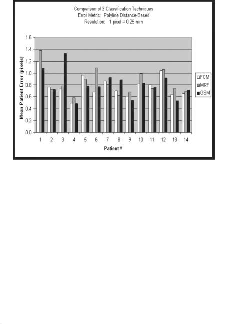
Figure 9.44: Results using FCM, MRF, and GSM methods.
9.6.2 Elliptical Binarization
The equations used for rotation of the ellipse about its center with an angle α is given by the new coordinates in Eq. (9.25).
xi |
= (xi − x0) cos(α) − (yi − y0) sin(α) |
(9.25) |
yi |
= (xi − x0) sin(α) − (yi − y0) cos(α) |
(9.26) |
9.6.3 Performance Evaluation of Three Techniques
Figure 9.44 shows the mean error bar charts for the three pipelines (i.e., using three classification systems: MRF, FCM, and GSM methods).5 The charts can be seen in the Tables 9.1–9.3. Table 9.1 shows the error between the computer-estimated boundary and ground truth boundary using FCM-based
5 We ran the system using each of the three different classifying methods on real patient data. Ground truth boundaries of the walls of the carotid artery were traced for 15 patients. Overall the number of boundary points was roughly 22,500 points. A pixel was equivalent to 0.25 mm. Using MRF, the average error was 0.61 pixels; using FCM, the average error was 0.62 pixels; using GSM, the average error was 0.74 pixels.

504 |
Suri et al. |
Table 9.1: Mean errors as computed using polyline and shortest distance methods when the classification system is FCM based
Patient No. |
Artifacted (PDM) |
Corrected (PDM) |
Artifacted (SDM) |
Corrected (SDM) |
|
|
|
|
|
1 |
2.052 |
1.195 |
2.063 |
1.216 |
2 |
0.928 |
0.764 |
0.948 |
0.794 |
3 |
3.174 |
0.729 |
3.180 |
0.756 |
4 |
1.106 |
0.490 |
1.118 |
0.513 |
5 |
1.514 |
0.968 |
1.529 |
0.993 |
6 |
1.079 |
0.681 |
1.094 |
0.704 |
7 |
1.278 |
0.863 |
1.310 |
0.893 |
8 |
0.928 |
0.695 |
0.944 |
0.723 |
9 |
0.758 |
0.606 |
0.783 |
0.631 |
10 |
1.004 |
0.813 |
1.027 |
0.840 |
11 |
1.407 |
0.808 |
1.418 |
0.826 |
12 |
1.408 |
1.042 |
1.426 |
1.078 |
13 |
0.735 |
0.643 |
0.753 |
0.670 |
14 |
0.922 |
0.655 |
0.939 |
0.685 |
|
|
|
|
|
method. Column 1 shows the error when the estimated boundary is not corrected (artifacted), using the PDM ruler. Column 2 shows the error when the estimated boundary is corrected by merging multiple classes of the lumen, using the PDM ruler. Column 3 shows the error when the estimated boundary is not corrected (artifacted), using the SDM ruler. Column 4 shows the error when the estimated boundary is corrected by merging multiple classes of the lumen, using the SDM ruler. As seen in the table, column 2 shows the least error and is significiantly improved over the artifacted boundaries. Table 9.2 shows the error between the computer-estimated boundary and ground truth boundary using MRF-based method. Column 1 shows the error when the estimated boundary is not corrected (artifacted), using the PDM ruler. Column 2 shows the error when the estimated boundary is corrected by merging multiple classes of the lumen, using the PDM ruler. Column 3 shows the error when the estimated boundary is not corrected (artifacted), using the SDM ruler. Column 4 shows the error when the estimated boundary is corrected by merging multiple classes of the lumen, using the SDM ruler. As seen in the table, column 2 shows the least error and is significiantly improved over the artifacted boundaries. Table 9.3 shows the error between the computer-estimated boundary and ground truth boundary using GSM-based method. Column 1 shows the error when the estimated boundary is not corrected (artifacted), using the PDM ruler. Column 2 shows the error when the estimated boundary is corrected by merging multiple classes of the lumen,

Lumen Identification, Detection, and Quantification in MR Plaque Volumes |
505 |
Table 9.2: Mean errors as computed using polyline and shortest distance methods when the classification system is MRF based
Patient No. |
Artifacted (PDM) |
Corrected (PDM) |
Artifacted (SDM) |
Corrected (SDM) |
|
|
|
|
|
1 |
1.609 |
1.382 |
1.627 |
1.402 |
2 |
0.831 |
0.726 |
0.857 |
0.759 |
3 |
1.174 |
0.781 |
1.195 |
0.805 |
4 |
0.687 |
0.584 |
0.706 |
0.605 |
5 |
1.239 |
0.895 |
1.263 |
0.917 |
6 |
1.164 |
1.086 |
1.182 |
1.105 |
7 |
1.100 |
0.807 |
1.124 |
0.839 |
8 |
1.004 |
0.620 |
1.023 |
0.645 |
9 |
0.696 |
0.679 |
0.714 |
0.702 |
10 |
0.890 |
0.958 |
0.912 |
0.982 |
11 |
0.938 |
0.736 |
0.954 |
0.763 |
12 |
0.941 |
1.065 |
0.965 |
1.089 |
13 |
0.679 |
0.740 |
0.704 |
0.761 |
14 |
0.851 |
0.694 |
0.869 |
0.716 |
|
|
|
|
|
Table 9.3: Mean errors as computed using polyline and shortest distance
methods when the classification system is GSM based
Patient No. |
Artifacted (PDM) |
Corrected (PDM) |
Artifacted (SDM) |
Corrected (SDM) |
|
|
|
|
|
1 |
1.081 |
1.081 |
1.105 |
1.105 |
2 |
0.721 |
0.721 |
0.746 |
0.746 |
3 |
1.329 |
1.329 |
1.351 |
1.351 |
4 |
0.487 |
0.487 |
0.505 |
0.505 |
5 |
0.778 |
0.778 |
0.802 |
0.802 |
6 |
0.767 |
0.767 |
0.788 |
0.788 |
7 |
0.920 |
0.920 |
0.949 |
0.949 |
8 |
0.885 |
0.885 |
0.903 |
0.903 |
9 |
0.536 |
0.536 |
0.559 |
0.559 |
10 |
0.826 |
0.826 |
0.849 |
0.849 |
11 |
0.752 |
0.752 |
0.774 |
0.774 |
12 |
0.914 |
0.914 |
0.942 |
0.942 |
13 |
0.533 |
0.533 |
0.557 |
0.557 |
14 |
0.708 |
0.708 |
0.732 |
0.732 |
|
|
|
|
|
using the PDM ruler. Column 3 shows the error when the estimated boundary is not corrected (artifacted), using the SDM ruler. Column 4 shows the error when the estimated boundary is corrected by merging multiple classes of the lumen, using the SDM ruler. As seen in the table, column 2 shows the least error and is significiantly improved over the artifacted boundaries.
506 |
Suri et al. |
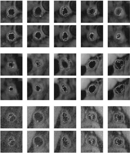
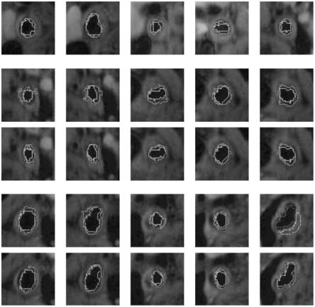
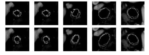
Figure 9.45: Results of estimated boundary using circularvs. elliptical-based methods. The system used was FCM based. Top rows are circular-based ROI, while the corresponding bottom rows are elliptical-based ROIs.
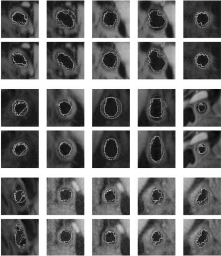
9.6.4 Visualization of Circular versus Elliptical Methods
Figures 9.45–9.48 show the comparision between the outputs of the systems when the system uses circular ROI versus elliptical ROIs. The visualization results from the two systems (one with circular ROI vs. elliptical ROI) are shown in pairs: top row corresponds to circular ROI methodology, while bottom row corresponds to elliptical ROI. Note that the equation for computing the elliptical ROI is shown in Eq. (9.25).
Lumen Identification, Detection, and Quantification in MR Plaque Volumes |
507 |
Figure 9.46: Results of estimated boundary using circularvs. elliptical-based methods. The system used was FCM based. Top rows are circular-based ROI, while the corresponding bottom rows are elliptical-based ROIs.
9.7 Conclusions
9.7.1 System Strengths
This chapter presented the following new implementations when it comes to MR plaque imaging: (a) Application of three different sets of classifiers for lumen region classification in plaque MR protocols. These classifiers are done in multiresolution framework. Thus subregions are chosen and subclassifiers are applied to compute the accuracy of the pixel values belonging to a class.
(b) Region merging for subclasses in lumen region to compute accurate lumen region and lumen boundary in cross-sectional images. (c) Rotational effect of
Lumen Identification, Detection, and Quantification in MR Plaque Volumes |
509 |
Figure 9.48: Results of estimated boundary using circularvs. elliptical-based methods. The system used was FCM based. Top rows are circular-based ROI, while the corresponding bottom rows are elliptical-based ROIs.
in most cases is the farthest distance from the center to a point on the contour. The ROI is the circle given by this center and this radius. The center and radius are sometimes adjusted after seeing the result of the pipeline’s first run.
9.8 Acknowledgments
The authors thank the Department of Radiology for the MR datasets. Thanks also to the students of Biomedical Imaging Laboratory at the Department of Biomedical Engineering, Case Western Reserve University for cooperating on sharing the calibrated machines for tracing the ground truth on plaque volumes.
Questions
1.What is arterial remodeling? (Lancet, Vol. 353, pp. SII5–SII9, 1999)
2.What are the main challenges in lumen quantification process?
3.Discuss the three types of algorithms used in this chapter for lumen estimation?
4.What brings the low error and why?
5.Compare the error performance using three different systems?

510 |
Suri et al. |
Bibliography
[1]Rogers, W. J., Prichard, J. W., Hu, Y. L., Olson, P. R., Benckart, D. H., Kramer, C. M., Vido, D. A., and Reichek, N., Characterization of signal properties in atherosclerotic plaque components by intravascular MRI, Arterioscler. Thromb. Vasc. Biol., Vol. 20, No. 7, pp. 1824–1830, 2000.
[2]Ross, R., Atherosclerosis—An inflammatory disease, N. Engl. J. Med., Vol. 340, No. 2, pp. 115–126, 1999.
[3]Reo, N. V. and Adinehzadeh, M., NMR spectroscopic analyses of liver phosphatidylcholine and phosphatidylethanolamine biosynthesis in rats exposed to peroxisome proliferators—A class of nongenotoxic hepatocarcinogens, Toxicol. Appl. Pharmacol., Vol. 164, No. 2, pp. 113– 126, 2000.
[4]Pietrzyk, U., Herholz, K., and Heiss, W. D., Three-dimensional alignment of functional and morphological tomograms, J. Comput. Assist. Tomogr., Vol. 14, No. 1, pp. 51–59, 1990.
[5]Coombs, B. D., Rapp, J. H., Ursell, P. C., Reily, L. M., and Saloner, D., Structure of plaque at carotid bifurcation: High-resolution MRI with histological correlation, stroke, Vol. 32, No. 11, pp. 2516–2521, 2001.
[6]Brown, B. G., Hillger, L., Zhao, X. Q., Poulin, D., and Albers, J. J., Types of changes in coronary stenosis severity and their relative importance in overall progression and regression of coronary disease: Observations from the FATS TRial: Familial Atherosclerosis Treatement Study, Ann. N.Y. Acad. Sci., Vol. 748, pp. 407–417, 1995.
[7]Helft, G., Worthley, S. G., Fuster, V., Fayad, Z. A., Zaman, A. G., Corti, R., Fallon, J. T., and Badimon, J. J., Progression and regression of atherosclerotic lesions: Monitoring with serial noninvasive MRI, Circulation, Vol. 105, pp. 993–998, 2002.
[8]Hayes, C. E., Hattes, N., and Roemer, P. B., Volume imaging with MR phased arrays, Magn. Reson. Med., Vol. 18, No. 2, pp. 309–319, 1991.
Lumen Identification, Detection, and Quantification in MR Plaque Volumes |
511 |
[9]Gill, J. D., Ladak, H. M., Steinman, D. A., and Fenster, A., Segmentation of ulcerated plaque: A semi-automatic method for tracking the progression of carotid atherosclerosis, In: Proceedings of 22nd Annual EMBS International Conference, 2000, pp. 669–672.
[10]Yang, F., Holzapfel, G., Schulze-Bauer, Ch. A. J., Stollberger, R., Thedens, D., Bolinger, L., Stolpen, A., and Sonka, M., Segmentation of wall and plaque in in vitro vascular MR images, Int. J. Cardiovasc. Imaging, Vol. 19, No. 5, pp. 419–428, 2003.
[11]Kim, W. Y., Stuber, M., Boernert, P., Kissinger, K. V., Manning, W. J., and Botnar, R. M., Three-dimensional black-blood cardiac magnetic resonance coronary vessel wall imaging detects positive arterial remodeling in patients with nonsignificant coronary artery disease, Circulation, Vol. 106, No. 3, pp. 296–299, 2002.
[12]Wilhjelm, J. E., Jespersen, S. K., Hansen, J. U., Brandt, T., Gammelmark, K., and Sillesen, H., In vitro imaging of the carotid artery with spatial compound imaging, In: Proceedings of the 3rd Meeting of Basic Technical Research of the Japan Society of Ultrasonic in Medicine, 1999, Vol. 15, pp. 9–14.
[13]Jespersen, S. K., Gro/nholdt, M.-L. M., Wilhjelm, J. E., Wiebe, B., Hansen, L. K., and Sillesen, H., Correlation between ultrasound B- mode images of carotid plaque and histological examination, IEEE Proc. Ultrason. Symp., Vol. 2, pp. 165–168, 1996.
[14]Quick, H. H., Debatin, J. F., and Ladd, M. E., MR imaging of the vessel wall, Euro. Radiol., Vol. 12, No. 4, pp. 889–900, 2002.
[15]Corti, R., Fayad, Z. A., Fuster, V., Worthley, S. G., Helft, G., Chesebro, J., Mercuri, M., and Badimon, J. J., Effects of lipid-lowering by simvastatin on human atherosclerotic lesions: A longitudinal study by high-resolution, noninvasive magnetic resonance imaging, Circulation, Vol. 104, No. 3, pp. 249–252, 2001.
[16]Fayad, Z. A. and Fuster, V., Characterization of atherosclerotic plaques by magnetic resonance imaging, Ann. N. Y., Acad. Sci., Vol. 902, pp. 173– 186, 2000.