Kluwer - Handbook of Biomedical Image Analysis Vol

542 Sato

where p, q, and r are nonnegative integers satisfying p + q + r ≤ 2. To obtain the normalized Gaussian derivatives, σ fp+q+r further needs to be multiplied with fxp yq zr (x" ; σ f ). In our experience, it is recommended that the radius of the kernel should be 3 · σ f , 4 · σ f , and 5 · σ f in simple smoothing ( p + q + r = 0), first ( p + q + r = 1), and second derivatives ( p + q + r = 2), respectively, for the accurate computation of the Gaussian derivatives and smoothing. Using this decomposition, the amount of computation needed can be reduced from O (n3) to O (3n), where n is the kernel diameter.

The eigenvalues were computed using Jacobi’s method in the simulations and experiments shown in this chapter. A numerical problem could exceptionally occur in this computation for synthesized images of the mathematical line models without noise. However, the numerical problem can be avoided by adding a very small Gaussian noise. We did not have such a numerical problem in the experiments using MR and CT images since noise is essentially involved in real images.

10.2.3.3 Guidelines for Parameter Value Selection

The multiscale enhancement filter includes several parameters. In defining the similarity measures to local structures, γst and α in Eqs. (10.3) and (10.4) need to be specified, while in the multiscale integration, the smallest scale σ1, the scale factor s, and the number of scale levels n in Eq. (10.17) need to be specified.

With regard to the parameters in the line measure, if there are strong sheet structures to be removed from an image, γ23 should be 1.0. If the cross sections of line structures of interest vary not only in size but also in shape, γ23 should be 0.5. γ12 also should be determined to optimize the trade-off between the preservation of branches and the reduction of noise and spurious branches. However, the performance has been found to be relatively insensitive to the values of γ23 and γ12 as long as they are between 0.5 and 1.0. Also, we have empirically found that α = 0.25 can be considered a good compromise.

With respect to the parameters in multiscale integration, we experimentally

√

found that s should be 1.5, 2, or less for reasonable approximation of the multiscale integration of the continuous scale. The minimum value of σ1 for discrete samples of volume data was 0.8 (voxels), which are experimentally shown in [7]. Considering the above observations, suitable values for σ1 and n should be found out for each case taking account of the anatomical structure of

interest based on the width response curves as shown in Fig. 10.3. We confirmed that the results were quite stable for different images obtained under similar conditions once suitable values have been determined.

The detailed analyses of the effects of parameter values on the filter responses, which are the bases of the above guidelines, are discussed for the line case in the next section, and more thorough analyses of them are found in [7].

10.2.4 Examples

10.2.4.1 Neurovascular Visualization from 3-D MR Data

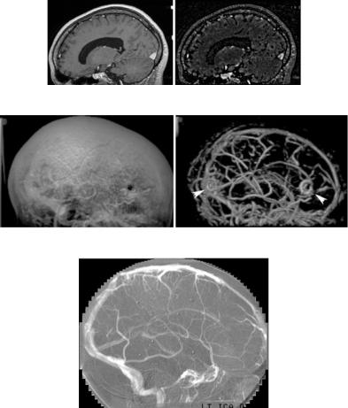
Multiscale line filtering was applied to postcontrast gradient-echo (SPGR) MR images of the brain for the purpose of vessel enhancement so as to use the enhanced vein structures as landmarks for brain tumor resection [26, 27]. The MRI dataset consisted of 192 sagittal slices of 256 × 256 pixels. The pixel dimensions were 1.0 mm2, while the slice thickness was 1.2 mm. The DSA images obtained from the same patient were also available, and used to compare with the vessel visualization with the MRI data. We used 80 slices corresponding to the right half of the head, and trimmed a region of 220 × 150 pixels from each slice. Sinc interpolation was performed for the trimmed images to obtain isotropic voxel sampling (the left frame of Fig. 10.4(a)). Multiscale line filtering was applied to the interpolated images using γ23 = γ12 = 1.0, α = 0.25, σ1 = 0.8 pixel, s = 1.5, and n = 3 (the right frame of Fig. 10.4(a)). The original and line-filtered images were visualized using the volume-rendering technique [28, 29] (Fig. 10.4(b)).

It is quite difficult to perceive the vessels through the skin in the volumerendered original images, but almost the same vein structures as in the DSA image (Fig. 10.4(c)) can be clearly seen in the volume-rendered line-filtered images. Although the vessels and the skin had almost the same intensity level in the original images, the line filter could mostly remove the effect of the skin since it has a sheet-like structure. As a side effect, the line filter also gave high levels of response to the rims of biopsy holes in the skin and skull. It is a current limitation of our formulation that the line filter gives a high level of response to rim structures as well as to line structures. In order to remove rim structures, a procedure such as the nonlinear combination of the first derivatives for line detection from 2-D images [3, 30], needs to be extended for use with 3-D images.

(a)

(b)

(c)

Figure 10.4: Neurovascular visualization from 3-D MR data. (a) Original (left) and line-filtered (right) cross-sectional images. (b) Original (left) and line-filtered (right) volume rendered images. (c) DSA (digital subtraction angiography) image at a vein phase.

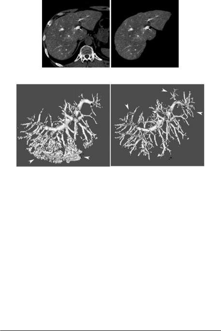
10.2.4.2 Portal Vein Segmentation from 3-D CT Data

Multiscale line filtering was applied to abdominal CT images taken by a helical CT scanner so as to segment the portal veins to localize a tumor with the relation to them for surgical planning. The CT dataset consisted of 43 slices of 512

× 512 pixels; the pixel dimensions were 0.59 mm2. The beam width was 3 mm and the reconstruction pitch was 2.5 mm. The CT data were imaged using CTAP

s = 1.5, and n = 2. We multiplied the mask images with the line-filtered images, thresholded the masked line-filtered images using an appropriate threshold value, and removed small connected components whose size was less than 10 voxels.

In Fig. 10.5(b), the left frame gives the rendered result of the original binary images, and the right frame shows a combination of the line-filtered binary images for small-vessel detection and the original binary images using relatively high threshold values for large-vessel detection. The two binary images were combined by taking the union of them. The CT data were scanned when the contrast material in the portal vein began to be absorbed by the liver tissues, as seen in the lower part of Fig. 10.5(b). Such a condition is quite common in CTAP for portal vein imaging. In the original images, the small vessels appear buried due to the contrast material absorbed by the liver tissue. In the combined result of the original and line-filtered images, not only is the nonuniformity of the contrast material canceled out, but also the recovery of small vessels is significantly improved over the entire liver area.

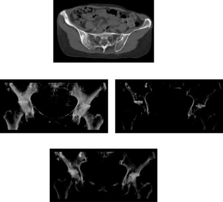
10.2.4.3Pelvic Bone Tumor and Cortex Visualization from 3-D CT Data

A single-scale sheet filter was applied to pelvic CT images for bone cortex enhancement. The purpose was to visualize the distribution of bone tumors and localize them in relation to the pelvic structure for biopsy planning as well as diagnosis [32]. Healthy bone cortex tissues and bone tumors have similar original CT values. However, bone cortices are sheet-like in structure, while tumors are not. Thus, enhanced bone cortices using sheet enhancement filtering are expected to be discriminated from tumors which are not enhanced.

The CT dataset consisted of 40 slices with a 512 × 512 matrix (Fig. 10.6(a)); the pixel dimensions were 0.82 mm2. The slice thickness and reconstruction pitch were 5 mm. The matrix was reduced to half in the xy-plane, and thus the pixel interval was 1.64 mm. Sheet filtering was applied to the sinc-interpolated images using σ f = 1.0 pixel, γ23 = γ13 = 0.5, and α = 0.25.

Figure 10.6(b) shows the color volume renderings of bone tumors (pink) and cortices (white). In the left frame, the opacity and color functions were adjusted using only CT values of the original images. In the right frame, both the original and sheet filtered images were used, where voxels having high intensities

(a)

(b)

(c)

Figure 10.6: Visualization of pelvic bone tumors from CT data. (a) Original CT slice image. (b) Volume rendered images of bone tumors and cortices. Left: Using only original images. Right: Using original and sheet-filtered images. (c) Manually traced tumor regions. ( c 2004 IEEE). A color version of this figure will appear on the CD that accompanies the volume.

both in sheet-filtered and original images were assigned as cortices (white), and those having high in original but low in sheet-filtered images were assigned as tumors (pink). Figure 10.6(c) shows the rendered color image generated from the tumor regions manually traced by a radiology specialist, which is regarded as an ideal visualization. The color rendering of the left frame of Fig. 10.6(b) was well correlated with Fig. 10.6(c) (the “ideal” image), and the bone tumors were visualized considerably better than only using original CT images. However, nontumor regions around articular spaces were also detected mainly due to the partial volume effect (by a large slice thickness).

(a)

(b)

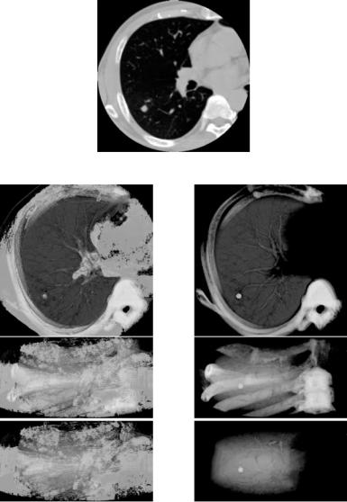
Figure 10.7: Visualization of lung nodule and vessel from CT data (Color Slide).

(a) Original CT slice image. (b) Volume rendered images of nodules (green), vessels (red), lung (violet), and bone (white) tissues. Left: Using only original images. Right: Using original, blob-filtered, and line-filtered images. ( c 2004 IEEE).

multiscale enhancement filters, simulation experiments were performed using synthesized images. In this section, the effects of parameter γ23, initial scale σ0, and scale factor s are presented based on simulations using a line model with an elliptic cross section. The effects of parameters γ12 and α are not presented here. Simulation experiments are presented in [7] to analyze the effects of parameters

γ12, and α using curved and branched line models.

10.3.1Single-Scale Filter Responses to Mathematical Line Models

The line measure generalizes λmin23 in Eq. (10.5) and λg−mean23 in Eq. (10.6). An alternative measure is to use the arithmetic mean of −λ2 and −λ3, which is given by

To compare these three measures, let us consider a 3-D line image with elliptic (nonisotropic Gaussian) cross sections given by

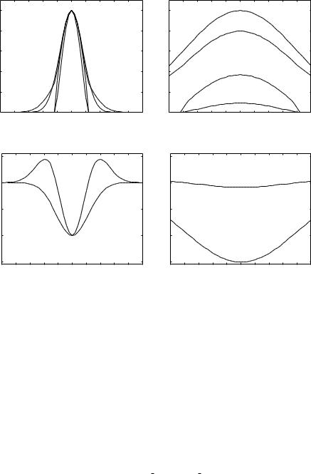
line(x" ; σx). Figure 10.8 shows the plots of the three measures and the eigenvalue variations of the Hessian matrix along the x-axis for the ideal line (σx = σy = 4 in Eq. (10.21), σ f = 4) and the sheet-like (σx = 20, σy = 3, σ f = 4) cases. The directions of the three eigenvectors at the points on the x-axis are identical to the x-axis, y-axis, and z-axis in the 3-D images modeled by Eq. (10.21). Let e"x, e"y, and e"z be eigenvectors whose directions are identical to the x-axis, y-axis, and z-axis, respectively, and let λx, λy, and λz be the respective corresponding eigenvalues. Figures 10.8(a) and 10.8(b) show the plots of λg−mean23 , λa−mean23 , and λmin23 as well as the original profiles, while Figs. 10.8(c) and 10.8(d) show the plots of λx, λy, and λz. In the ideal line case, both λ2 and λ3 are negative with large absolute values near the line centers. Since λ3 tends to have a larger absolute value in the sheet-like case than in the line case (Fig. 10.8(d)), λa−mean23 still gives a high response in the sheet-like case even if λ2 has a small absolute value. Figure 10.9 shows the responses of the three measures at the center of