Kluwer - Handbook of Biomedical Image Analysis Vol

We define the height measure of the multiscale filter response as the peak response hM(σr ) = Mline{ line(0, 0, z ; σr )}. Since the filter response is normalized, hM(σr ) is constant regardless of σr . That is,

where hMc = 0.25 (see the “Brain Storming Question” at the end of this chapter

for the derivation). We define the width measure wM(σr ) of the multiscale filter

response as the distance x02 + y02 from the z-axis to the circular locus where

Mline{ line(x0, y0, z ; σr )} gives half of the peak response, that is, hM2 c . Let wM(σr ) be the ratio of the observed width wM(σr ) to σr . The width ratio wM(σr ) is constant regardless of σr , that is,

where wMc ≈ 1.0 when γ 23 = 1 in the formulation of Eq. (10.2). Similarly, we define the height measure hR(σr ; σ f ) of the single-scale filter response as the

peak response hR(σr ; σ f ) = Sline{ line(0, 0, z ; σr ); σ f } and the width measure

wR(σr , σ f ) as the distance x02 + y02 from the z-axis to the circular locus where

Sline{ line(x0, y0, z ; σr ); σ f } gives the half of the maximum response, hM2 c . To compare the widths of the filter response and the original profile, we also in-

troduce the width measure wL(σr ) of the original line image as the distance

x02 + y02 from the z-axis to the circular locus where line(x0, y0, z; σr ) gives half of line(0, 0, z ; σr ). While σr is introduced for the convenience of generating line profiles, wL(σr ) is for the convenience of comparing the widths of various profile shapes.

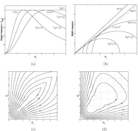
Figure 10.10(a) and 10.10(b) show the variations in the height and width measures. Figure 10.10(a) gives the plots of hR(σr ; σ f ) at three values of σ f and hM(σr ), and Fig. 10.10(b) shows the plots of wR(σr ; σ f ) at three values of σ f , wM(σr ), and wL(σr ). The width measure of the multiscale response is proportional to that of the original line image. In the case of the line image line(x" ; σr ) with a Gaussian cross section, wL(σr ) ≈ 0.9wM(σr ). Although the filter responses make the lines a little thinner than the original lines, the multiscale line-filter can be designed so that the width of its responses becomes approximately proportional to the original one.

values of σ f . In 3-D image filtering, a large amount of computation is necessary to obtain the filter response at each value of σ f . The maximum and minimum values of σ f can be essentially determined on the basis of the width range of the anatomical structure of interest. The interval of σ f should be sufficiently small for the filter response to work uniformly for every line width within the width range, while it is desirable that it should be large enough to minimize the amount of computation required. Thus, we need to determine the minimum number of discrete samples of σ f which satisfy the following conditions:

1.The height measure of the response should be approximately constant within the width range.

2.The width measure of the response should be approximately proportional to the original one within the width range.

Given the discrete samples of σ f and the assumption of the cross-section shape (here, we use the Gaussian cross section), the accuracy of the approximation can be estimated. Let σi = si−1σ1 (i = 1, 2, . . . , n) be discrete samples of σ f , where σ1 is the minimum scale and s is the scale factor determining the sampling interval of σ f . The multiscale filter response using the discrete samples of σ f is given by

where σi = si−1σ1 (i = 1, 2, . . . , n), hMmin is the minimum of the height measure of the multiscale response Mline{ line(x", σr )} within the range kpσ1 ≤ σr ≤ kpsnσ1, and the minimum is taken at σr = kpsiσ1 (i = 0, 1, 2, . . . n) (Fig. 10.10(a)). hMmin can be regarded as a function of the scale factor s. The height measure of the multiscale response should be sufficiently close to hMc within the width range of interest. The values of hMmin and kp at typical scale factors are summarized in

γ 23 = 0.5, respectively. The multiscale integration of these discrete scales gives a good approximation of that of the continuous scales.

10.4 Description and Quantification

In the previous sections, the enhancement of the local structures based on the eigenvalues of the Hessian matrix was discussed. In this section, we further combine the gradient vector with the Hessian matrix to perform explicit detection, localization, and description of the local structures. Especially, we focus on the line and sheet structures. The methods are formulated as a 3-D extension of 2-D line description presented in [36]. The 3-D line model consists of the medial axes of lines and the cross-sectional shape associated with each point on these axes, while the 3-D sheet model consists of the medial surfaces of sheets and the width associated with each point on these surfaces. The medial axes and medial surfaces are detected and localized by fully utilizing formal analyses of 3-D second-order local intensity structures based on the gradient vector and the Hessian matrix.

The following is an overview of the method:

Step 1: Existing filtering techniques for line and sheet enhancement are used to extract the initial regions, which should include all potential medial axes and surfaces [7, 11]. These are then used as initial values for the subsequent subvoxel edge localization. The candidate regions, which should include all potential line and sheet regions, are also extracted.

Step 2: The medial axes and surfaces are extracted using local secondorder approximation given by the gradient vector and Hessian matrix. The eigenvectors of the Hessian matrix define the moving frames on medial axes/surfaces. After this, the moving frames are embedded in a 3-D image such that each point within the candidate regions is directly related to its corresponding moving frame.

Step 3: Subvoxel edge localization of the region boundaries is carried out using adaptive 3-D directional derivatives, whose directions are adaptively changed depending on the moving frame, to accomplish accurate segmentation, model recovery, and quantification.

In the following, we begin with a description of Step 2 of the method since Step 1 has been already described in the previous sections.

10.4.1 Medial Axis and Surface Detection

Let f (x") be an intensity function of a volume, where x" = (x, y, z), and f (x" ; σ ) be its Gaussian smoothed volume with standard deviation σ . The second-order

where f0 = f (x"0), f 0 = f (x"0), and 2 f 0 = 2 f (x"0). Thus, the second-order structures of local intensity variations around each point of a volume can be described by the original intensity, the gradient vector, and the Hessian matrix.

The gradient vector of Gaussian smoothed volume f (x" ; σ ) is defined as

Let the eigenvalues of 2 f (x" ; σ ) be λ1, λ2, λ3 (λ1 ≥ λ2 ≥ λ3) and their corresponding eigenvectors be e"1, e"2, e"3 (|"e1| = |"e2| = |"e3| = 1), respectively. For the ideal line, e"1 is expected to give its tangential direction and both |λ2| and |λ3|, directional second derivatives orthogonal to e"1, should be large on its medial axis, while e"3 is expected to give the orthogonal direction of a sheet and only |λ3| should be large on its medial surface (Fig. 10.11). Here, structures of interest are assumed to be brighter than surrounding regions.

The initial regions obtained in Step 1 are searched for medial axes and surfaces, which are detected based on the second-order approximation of f (x" ; σ ) The medial axis and surface extraction is based on a formal analysis of the second-order 3D local intensity structure. Here, σ f is the filter scale used in

Figure 10.11: Line and sheet models with the eigenvectors of the Hessian matrix. (a) Line. (b) Sheet.

medial axis/surface detection, and we assume that the width range of structures of interest is around the width at which the filter with σ f gives the peak response (see [7] and [11] for detailed discussions).

10.4.1.1 Line Case—Medial Axis Detection

We assume that the tangential direction is given by e"1 at the voxel around the medial axis. The 2-D intensity function, c(u") (u" = (u, v)$), on the cross-sectional plane of f (x" ; σ f ) orthogonal to e"1, should have its peak on the medial axis. The second-order approximation of c(u") is given by

that is, f (x"0; σ f )), and

c(u") should have its peak on the medial axis of the line. The peak is located at the position satisfying

The territory of the detected point in the Voronoi tessellation can be regarded as the set of voxels to which each discrete moving frame is applied. This process is identical in both the line and sheet cases.

10.4.2Subvoxel Edge Localization and Width Measurement

An adaptive directional second derivative is applied at each voxel based on its corresponding moving frame. The directional derivative is taken along the perpendicular from the voxel to the medial axis or surface. The zero-crossing points of the directional second derivatives are localized at subvoxel resolution to determine the precise region boundaries and quantitate the widths.

At every voxel within the candidate regions, the directional second derivative is calculated depending on its corresponding moving frame. This spatially variable directional derivative is written as

where r"(x") is the unit vector whose direction is parallel to the perpendicular from the voxel position x" to the straight line defined by the origin and the medial axis direction of the moving frame. The foot of the perpendicular can be regarded as the corresponding axis position. The origin is given by the voxel position of the medial axis point and the offset vector p". σe is the filter scale used in the edge localization; it is desirable that σe be small compared to the line width for accurate edge localization.

After the adaptive derivatives have been calculated at all the voxels, subvoxel edge localization is carried out at every voxel in the candidate regions. Let o"a be the foot of the perpendicular on the axis. Let r"a be the direction from o"a to the voxel position x"a. For each voxel, we reconstruct the profiles originating from o"a in the directions r"a and −r"a for fline(x" ; σe) and the initial regions (which we specify as bline(x")) obtained in Step 1. The edges are then localized in both directions and the width is calculated as the distance between the two edge locations. The profile is reconstructed at subvoxel resolution by using a trilinear interpolation for fline(x" ; σe) and a nearest-neighbor interpolation for bline(x").

Let f (s) be the profiles of fline(x" ; σe) along the directions r"a from o"a. Let b(s) be the profiles of bline(x"). Here, r denotes the position from the foot of