Kluwer - Handbook of Biomedical Image Analysis Vol

each expert, p(r), are determined in an unsupervised manner through statistical methods.

11.4.4.3.1 Maximum Likelihood Solution. The mixing coefficient parameter values for each expert can be determined using the ML principle by forming a likelihood function. Assume that we have the complete dataset, ψ , of combined decisions from segmentation experts for each data point, where

ψ = {yˆ1, . . . , yˆ N ), and it is drawn independently from the complete distribution p(yˆ | x, ). Then the joint occurrence of the whole dataset is given as

n=1 r=1

For simplicity, the above likelihood function can be rewritten and expressed as a log likelihood as follows:

For the above equation, it is not possible to find the ML estimate of the parameter values directly because of the inability to solve = 0 [23]. Our approach used to maximising the likelihood log ζ ( ) is based on the EM algorithm proposed in the context of missing data estimation [35].

11.4.4.3.2 AWM Parameter Estimation Using EM Algorithm. The EM algorithm attempts to maximize an estimate of the log likelihood that expresses the expected value of the complete data log likelihood conditional on the data points. By evaluating an auxiliary function, Q in the E-step, an estimate of the log likelihood can be iteratively maximized using a set of update equations in the M-step. Using the AWM likelihood function from Eq.(11.30) the auxiliary function for the AWM is defined as

n=1 r=1

It should be noted that the a posteriori estimate p(yˆn | r, xn) for the nth data point from the rth segmentation expert remains fixed. The conditional density function pold(r | yˆn) is computed using the Bayes rule as

In order to maximize the estimate of the likelihood function given by the auxiliary

function, update equations are required for the mixing coefficients. These can be

obtained by differentiating with respect to the parameters set equal to zero. For

the AWM, the update equations are taken from [27]. For the rth segmentation

expert

The complete AWM algorithm is shown below.

Algorithm 2: AWM ALGORITHM

ter in turn:

1. The new estimate of the segmentation expert weightings for the rth component P new(r) is given by Eq.(11.33).

11.4.4.3.3 Estimating the A Posteriori Probability. Using the AWM

combination strategy in mammographic CAD, a posteriori estimates are re-

quired for each data point following the experts’ combination (one for the nor-

mal and one for the suspicious class). To determine these estimates, the AWM

model is computed for the first class, thereby obtaining the a posteriori estimate

p(yˆn = ω1 | xn, ). From this, the estimate of the second class is determined as p(yˆn = ω2 | xn, ) = 1 − p(yˆn = ω1 | xn, ). We now proceed to the results

section to evaluate our novel contributions of weighted GMM segmentation experts and the novel AWM combination strategy.

11.4.5Results of Applying Image Segmentation Expert Combination

The aim of our experiments was to (i) perform a comparison between the four proposed models of image segmentation. The baseline comparison with a simple GMM based image segmentation and an MRF model in [18] shows that our proposed models easily outperform the baseline models. (ii) To compare the performance of the AWM combination strategy against the ensemble combination rules. Section 11.4.5.1 compares the four models on the two databases, and section 11.4.5.2 compares the AWM approach with ensemble combination rules approach on the two databases.

Our segmentation performance evaluation is performed on 400 mammograms selected from the DDSM. The first 200 mammograms contain lesions and the remaining 200 mammograms are normal (used only for training purposes). Each of these mammograms has been categorized into one of the four groups representing different breast density, such that each category has 100 mammograms. The partitioning of the mammograms has been performed manually on the basis of the target breast density according to DDSM ground truth. The results will be reported in terms of the Az value that represents the area under the ROC curve as well as sensitivity (the segmentation evaluation for testing is based on ground-truth information as given in DDSM).

The grouping of mammograms by breast density is applicable only to the supervised approaches. Supervised approaches segmenting a mammogram with a specific breast density type use a trained observed intensity model constructed with only training samples from that breast type. Thus, each trained observed intensity model will be specialized in the segmentation of a mammogram with a specific breast type. We adopt a fivefold cross-validation strategy. Using this procedure, a total of five training and testing trials are conducted, and each time the data appearing in training does not appear as testing. For each of the fivefolds, equal numbers of normal and suspicious pixels are used to represent training examples from their respective classes. These sample pixels are randomly sampled from the training images. In the unsupervised

Winning strategies are given in bold.

case, there is no concept of training and testing and each image is treated individually.

11.4.5.1Comparison of the Four models

(WGMMS, WGMMU , WGMMMRFS , and WGMMUMRF)

A cross-validation approach is used to determine the optimal number of component Gaussians, for each breast type. The determined value of mis then used for all training folds comprising each breast type. To determine the optimal value of m, models with a different number of components are trained and evaluated with a WGMMS strategy, using an independent validations set. Model fitness is quantified by examining the log likelihood resulting from the validation set. Training files are created by taking 200 samples randomly drawn with replacement from each normal and abnormal images for each breast type. For training we use 50 training images per breast type (n = 25 normal, n = 25 abnormal) giving a training size of 10,000 samples per breast type. Repeating the procedure for 50 remaining validation image per breast type, we get 10,000 samples for validation.

In our evaluation procedure the aim is to determine the correct number of true positives (TP), false positives (FP), true negatives (TN), and false negatives (FN) in order to plot the ROC curve. A detailed summary of how each segmented region is classed as one of these is detailed in [18]. The results are shown in Table 11.10 grouped on the basis of breast density. It is easily concluded that the supervised strategy with MRF is a clear winner. Interestingly, the performance of this method is superior for denser images compared to fatty ones. A simple

explanation for this phenomenon could be based on the model order selection where m = 1 for the abnormal class of the fatty breast types. A more sophisticated approach to determining model order might improve the segmentation of these breast types. Without the hidden MRF model, the supervised strategy is inferior to the unsupervised approach on the denser breasts.

11.4.5.2Comparison of Combination Strategies: Ensemble Combination Rules vs. AWM

In order to develop a number of experts that can be combined, we extract different gray-scale and texture data per pixel in the images. The gray-scale values of the pixels are intensity values, and texture features are extracted from pixel neighborhood. The following table shows the different feature experts used in our analysis based on different features. Each expert can be implemented with one of the four segmentation models described earlier.

We now present the results on 200 test mammograms that contain lesions. The details of training and testing scheme are the same as detailed in section 11.4.2. As we mentioned earlier, each breast is classified as one of the four types (1, predominantly dense; 2, fat with fibroglandular tissue; 3, heterogeneously dense; and 4, extremely dense) and the results are presented for data from each type. Table 11.11 shows the test results on sensitivity of the

SEGMENTED IMAGES

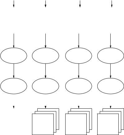
Figure 11.7: Schematic overview of false-positive reduction strategy within the

adaptive knowledge-based model.

11.5A Framework for the Reduction of False-Positive Regions

This section describes the approach used within the adaptive knowledge-based model for the reduction of false-positive regions. Figure 11.7 shows a schematic overview of the approach adopted. Using the actual breast type grouping predicted by the breast classification component, a segmented mammogram is directed to one of four process flows. Each process flow, shown in Fig. 11.7,

comprises the same functionality. This is discussed in more detail in the following subsections.

11.5.1Postprocessing Steps for Filtering Out False Positives

11.5.1.1 Region Prefiltering

Feature extraction is computationally expensive. A common strategy [6, 7, 36] to reduce the number of regions considered for false-positive reduction is achieved by applying a size test. By eliminating suspicious regions smaller than a predefined threshold Tarea, the number of false-positive regions can be reduced. For the expert radiologist interpreting a film mammogram during screening, it is common to disregard any suspicious ROI less than 8 mm in diameter [37]. In mammographic CAD with computer automation, the size threshold is reduced and a common value for Tarea is the number of pixels corresponding to an area of 16 mm2 [6, 7, 36]. In the adaptive knowledge-based model, the area threshold is set at 19.5 mm2 corresponding to a region diameter of 5 mm for all breast type groupings. The DDSM used in this evaluation are digitized such that each pixel is 50 m. Following subsampling by a factor of four, an area threshold of 19.5 mm2 is equivalent to Tarea = 122 pixels, thus any suspicious region following segmentation with an area less than this value is marked as normal.

11.5.1.2 Feature Extraction

Features are extracted to characterise a segmented region in the mammogram. Feature vectors from masses are assumed to be considered different from normal tissue, and based on a collection of their examples from several subjects, a system can be trained to differentiate between them. The main aim is that features should be sensitive and accurate for reducing false positives. Typically a set or vector of features is extracted for a given segmented region.

From the pixels that comprise each suspicious ROI passing the prefiltering size test described above, a subset of gray scale, textural, and morphological features used in previous mammographic studies are extracted. The features extracted are summarized in Table 11.14.

Table 11.14: Summary of features extracted by feature grouping giving 316 features in total

11.5.1.3 Principal Component Analysis

The result of feature extraction is a 316-dimensional feature vector describing various gray-scale histogram, textural, and morphological characteristics of each region. The curse of dimensionality [27] is a serious constraint in many pattern recognition problems and to maintain classification performance, the dimensionality of the input feature space must be kept to a minimum. This is especially important when using an ANN classifier, to maintain a desired level of generalization [32]. Principal component analysis (PCA) is a technique to map data from a high-dimensional space into a lower one and is used here for such a purpose.

To use PCA in the adaptive knowledge-based model in an unbiased way, the PCA coefficients, comprising eigenvalues and eigenvectors, are determined from an independent training set. In mapping to a lower dimensionality, only eigenvalues ≥ 1.0 are considered and the eigenvectors from training are applied to a testing pattern. Testing and training folds are formed using 10-fold cross validation [32] such that an unbiased PCA transformation can be obtained for each testing sample.