Kluwer - Handbook of Biomedical Image Analysis Vol

Table 13.1: BIRADS descriptors for calcifications with associated genesis

type [26]

B = probably benign; M = suggestive of malignancy; U = uncertain.

management. To be clinically useful, the algorithm should perform real time, be robust, and have consistent performance at least comparable to the clinical visual analysis system [20, 22]. The algorithm described here was designed to meet the above requirements and two additional conditions: (a) The desired classification performance had to be achieved with the smallest possible set of features. (b) Feature selection would be initially limited to the morphological, distributional, and demographic domains; expansion to other domains would be considered only if performance did not reach desirable levels. The specific components of this scheme are shown in Fig. 13.3. The algorithm was implemented and tested on simulated calcification clusters, large sets of mammographic calcifications, and datasets of various image resolutions [20, 28, 29]. All studies demonstrated that the development of a classifier on morphological characteristics alone is a viable and reliable approach. They also supported our hypothesis

Figure 13.3: Flowchart of the CADiagnosis algorithm developed for the differentiation of benign from malignant microcalcification clusters in digitized, screen/film mammography [20].

that a classifier could be used as an indirect measure of segmentation performance [29]. The segmentation of the individual calcifications and the clusters with shape and distribution preservation was a critical stage in our methodology. Hence, in the following section, we will discuss the detection/segmentation stage in more detail with particular emphasis on the role of wavelets in this process.

13.3 Detection/Segmentation Stage

The terms segmentation and detection may be confusing for the reader not so familiar with the medical imaging vernacular. In some instances these terms may be used interchangeably, but other times not. We might consider segmentation as being a more refined or specialized type of detection. For instance, we may gate a receiver for some time increment and make a decision as to whether or not a signal of interest was present within the total time duration, but not care about exactly where the signal is within the time window; this may be defined as a detection task with a binary output of yes or no. Segmentation takes this a step further. With respect to the image processing, the detection task makes a decision if the abnormality is present, which in this case is a calcification. If, in addition, the detection provides some reasonable estimate as to the spatial location and extent of the abnormality, then we would say that the calcification

has been segmented. Thus, the segmentation process in mammography often results in a binary-labeled image with the probable calcification areas marked.

Before getting into the details of the techniques we implemented for the detection/segmentation stage of our CADiagnosis algorithm, a brief discussion of related bibliography is in order for the novice or beginner in the field to allow for a heads-up on study material of the suitable level. The list that follows is in no-way complete, or totally contemporary, but is comprised of useful citations (textbooks generally) that we have used extensively in our research and algorithm development.

Tolstov [30], Bracewell [31], and Brigham [32] are excellent sources for studying Fourier series and Fourier transforms—a prerequisite to understanding the wavelet transforms used in our approach. In particular, Brigham [32] provides a comprehensible treatment of the relations with the continuous Fourier transform, the discrete Fourier transform, and sampling theory. Similarly, Bracewell [33] gives a well-balanced treatment of standard imaging processing techniques.

Noise and filtering will be discussed in the following sections. Generally, the study of noise processes comes under many subject headings such as stochastic analysis, random signal analysis, or probability analysis. Again there are many diverse resources in this area and several provide many useful examples of random variable transformations and Fourier analysis of random signals [34– 37]. An excellent treatment of transforms and probability analysis applications is given by Giffin [38].

Wavelet analysis may be looked at from a simple filtering approach as well as from an elegant mathematical framework that involves understanding multiresolution functional spaces. Again, there is massive published work in this area. Strang and Nguyen [39], Akansu and Haddad [40], and Vetterli and Kovacevic [41] are excellent sources for understanding wavelets from a filtering approach, which also include the multiresolution framework. The seminal work in wavelet theory may be found in the more mathematically sophisticated work of Daubechies [42].

Finally, in the sections below, we will discuss how mammograms are associated with power spectra that obey an inverse power law. This characteristic is associated with self-similarity, fractals, and chaos. We are not aware of any traditional textbooks that address power laws specifically but the work of Peitgen et al. [43], Wornell [44], and Turner et al. [45] may be useful; Peitgen et al. [43] cover many types of phenomena, while Wornell [44] and Turner et al. [45] are

specific to wavelet-based signal processing and 2-D image analysis, respectively. Note that the idea of self-similarity implies that things or events are invariant under a scale change. Wavelets have this property. Thus, it would seem natural to study self-similar noise fields (such as mammograms) with a self-similar analyzing transform (wavelets).

13.3.1 Wavelet Filtering

The term image enhancement is also a very general term, which encompasses many techniques. We have recognized that it is often used to describe the outcome of filtering. If the definition of enhancement is applying a process to the image that results in a “better” overall image appearance, then the term is a misnomer. Linear filtering blocks a portion of the true signal in most applications, which is probably not best defined as enhancement. In this section we provide a qualitative description of filtering. The only assumption we make here is that the reader understands Fourier analysis in one dimension. If so, the extension to two dimensions will be easily accomplished.

Things that change rapidly in the signal domain give rise to larger amplitudes for the sine waves that wiggle more quickly (high frequencies) in the Fourier expansion of the signal. Likewise, things that have long-range structure in the signal domain, give rise to larger amplitudes for the sine waves that wiggle slowly (low frequencies) in the Fourier expansion. Of course, there are many structures that lie in the middle of these extremes. The reader should keep in mind that the above descriptors are relative terms. Signals that are delta-function like will give rise to Fourier components across the entire spectrum. There is more to the story, because we are working in two dimensions. Let’s consider a two-dimensional function or contrived image that is nothing more than an infinite vertical line (y-direction) of a few pixels in width in the other direction (x-direction) embedded in an empty 2-D field. Note that in the vertical direction there is no variation along the line indicating it will look as a low frequency signal in this direction (this may be considered as a sine wave with an infinite period, which may be considered as a DC component). If we approach this line from the horizontal direction, it appears as an abrupt change, for an instance, then it is flat for a few pixels, then another abrupt change takes place, and it is gone; that is, any horizontal slice will look like the rectangle function that is used in many Fourier analysis textbooks for examples. It takes two frequency coordinates to describe

this signal or any 2-D signal (image). Specifically, this signal is purely a DC signal in the y-direction when considering its Fourier composition and a sinc-type function in the other direction. Consequently, the transform is a sinc function along the fx coordinate axis and about zero elsewhere; this may be deduced by considering the ( fx, fy) coordinates and noting that the fx component is zero everywhere except at fy = 0. The following may be observed: (1) Linear structures in the vertical direction are likely to give rise to Fourier signatures in the fx direction. The narrower the width the more spread out the contribution is in the Fourier fx direction and the wider in width, the more contracted along the fx direction. (2) Linear structures in the horizontal direction are likely to have significant Fourier signatures in the fy direction and less in the fx direction.

(3) Taking this a step further, spots give rise to components in both coordinate directions. These examples are idealizations that may inspire the newcomer to Fourier analysis to observe what exactly the Fourier Transform is telling the user.

Filtering can be applied to set the stage for detection or segmentation. The basic idea is that there is some structure that we define as the signal of interest, which in our case is the localized calcified areas in mammograms termed “calcifications.” These signals are surrounded (or embedded in) by other signals (in this case normal breast tissue) that may interfere with the ability to automatically detect them. In the best scenario, the signal of interest will have a frequency signature that is somewhat different than the background. If this is the case, filtering the image will pass the signal of interest (perhaps not intact) and block a portion of the background tissue. If this is successful, the filtered image will show a relatively more pronounced calcified area and a somewhat subdued background when compared with the raw image.

A simple somewhat contrived example of the usefulness behind filtering is proved here. Suppose we have a white 2-D (n × n) noise field with variance σ 2 and filter it with a perfect band pass filter. Can we say anything about the resulting noise power? The answer is yes. White noise by definition is a flat power spectrum (more correctly a constant power spectral density). For illustration, we will apply a perfect half-band filter to this field and calculate the resulting noise power. In the Fourier domain, the half band filter looks like a square box centered about zero of unit height with its sidewalls intersecting the frequency coordinates and the midway point. Fourier components within the box are passed when filtering and everything outside is blocked. Thus the total area in the Fourier domain is n2, the pass-band area is (n/2)2, and the blocked portion of

the Fourier domain is n2 − (n/2)2 = 34 n2. Considering the transform properties, the resulting noise power is 34 σ 2. The important point here is that if the signal of interest has strong signatures in the lower part of the frequency spectrum, they will be passed almost intact while the noise would be heavily damped. This is an idealized situation that helps to understand the reasons for filtering.

In the following, a very brief description of wavelet analysis is presented. There is no way that we can give proper justice to this elegant theory of signal decomposition. Beware it took great minds many years to put wavelet analysis on such a beautiful foundation, which is now discussed as commonplace.

When considering the actual wavelet application, the wavelets are not expressed explicitly in an analytical form, but are expressed as two filter kernels corresponding to a weighted differencing operator and a weighted smoothing operator, which are complementary operators. In the literature these are referred to as the mother wavelet and associated scaling function. The forward transform is applied by alternative applications of the two kernels with down sampling interleaved between the applications. This procedure generates the wavelet expansion coefficients. The inverse transform is also achieved by repeated convolutions with two related filter kernels with up-sampling interleaved between the convolutions. The filtering aspect of the analysis is implemented by applying the forward transform and setting the desired coefficients to zero before applying the inverse transform.

The procedure described above may also be presented using the equivalent terms of dilation (or contraction) and translation of the mother wavelet function. For a given wavelet basis, there is really only one wavelet function or mother wavelet. The entire basis is constructed from translations and dilations of this wavelet. Spreading it out reduces the resolution and translating provides spatial information. The translations and dilations are not arbitrary, but are picked in a certain way from an orthogonal basis at multiple resolutions.

A way to view this is that the wavelet coefficients are really correlation figures of merit indicating how well the signal and a given region correlates with the particular version of the mother wavelet. The important thing to note here is that when the wavelet is spread out, the inner product with the signal at a given region (or spatial location) encompasses the length of the dilated wavelet. This implies that the wavelets coefficient holds information about the entire spatial region. As the wavelet spreads out, the frequency-band narrows. Thus, the analysis is better localized in frequency but worse localized in space.

There are many orthogonal wavelet coefficients to choose from, and the band pass nature is not generally sharp indicating that the expansion components will have some shared frequency attributes; these cancel when performing the addition. Here is a simple rule of thumb: the shorter the wavelet filter kernel the less sharp the cutoffs are in the Fourier domain and the longer the support length the sharper the cutoffs. The strength of the two-channel or quadrature wavelet filter is the orthogonality of the expansion images. The price paid for orthogonality is the fixed-way the associated information is divided (octave sectioning).

13.3.2 Symmlet Wavelet Approach

As stated, there are many wavelet bases that can accomplish the detection and segmentation of calcified areas in mammogram and set the stage for the classification task. In a first application, we used a nearly symmetric wavelet. Our choice was guided by the close similarity between the wavelet profile and the calcification profiles (recall the correlation idea discussed above). First, the image is expanded as in Eq. (13.1). Deciding which components to discard is the crucial decision with this approach. This choice is dependent upon the calcification size (in both pixel width and actual linear measure) and the digital resolution. The term size is used in the average or expected sense. From the clinical view of a suspicious abnormality, calcifications of up to 1/2 mm are important. This translates into about 8–16 pixels in an image generated with a 35 m/pixel digital resolution; our original work was performed at this high resolution and this experience will be discussed here [46]. In pilot studies, the d3 and d4 images demonstrated the largest calcification signatures relative to the background and were empirically selected for the process. Two pathways could be followed: (1) Add the two relevant expansion images together and perform the detection or (2) perform the detection in each image and combine the results afterwards. The latter option gave better sensitivity performance, since it gives the opportunity to detect some calcified areas twice. Specifically, small calcifications had a stronger signature in the d3 images and large calcifications had stronger signatures in the d4 images. Many calcifications had of course signatures spread across the two components.

Rather than impose a detection or decision rule on the process, we decided early on to see whether a parametric approach to decision making could be followed. Our pilot studies showed that the wavelet expansion images could be

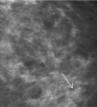
Figure 13.5: Representative mammographic section (2048 × 2048 pixels) with a malignant calcification cluster indicated by arrow. Image resolution is 35 m and 12 bits/pixel.

approximated with parametric methods to characterize their empirical pixel distributions [46–48]. Calcifications, and calcification clusters, occupy a relatively small portion of the image when present; Fig. 13.5 shows a typical calcification cluster associated with cancer. Given the small area properties, the wavelet modeling produced essentially the parametric probability distribution functions (PDF) for normal tissue at multiple resolutions.

Theoretically, knowledge of the surrounding tissue PDF allows for the development of a statistical criterion to test against it using maximum likelihood analysis [49]. Our work indicated that the PDFs may be approximated from a family of parametric PDFs indexed by N; when N = 1, the PDF is Laplacian, and when N is large it tends to a normal distribution and the PDF is symmetric about the origin (zero mean).

We will not delve into this area of statistics here, but will indicate the approximations used. In this application, we ignored the pixel correlation within

a given expansion image and used a low order N approximation. Namely, if N is in the neighborhood of 3, the N = 1 approximation was applied to simplify the techniques. Likewise, before applying the maximum likelihood analysis, the expansion images where transformed to all positive values by taking the absolute value. Figure 13.6 shows the first three wavelet expansion images for the mammogram of Fig. 13.5.

Knowing the form of the PDF allows for the development of a test statistic, better described as a summary statistic, which follows from the maximum likelihood approach. However, the technique does not indicate how exactly to apply the test to the problem at hand. The maximum likelihood analysis indicated that the average was the test statistic. Tailoring this to our problem translated into sliding a small search window across the image matched in size to the expected calcification size. At each location the average was calculated, and if the local average deviated from the expected overall normal tissue average, it was labeled as suspicious and marked. Otherwise, the local region was set to zero. Thus, by systematically analyzing each local image region, most of the image was discarded and the potential abnormalities were labeled. A different search size window was used for the different images: an 8 × 8 pixel window was applied to the d3 image and a 16 × 16 pixel window was applied to the d4 image. The detection result yielded two binary images that for the most part were zero but were equal to 1 in areas corresponding to calcifications. The union of the two detections formed the initial total binary detection output. But detecting isolated calcifications was not the end of the process. Calcifications had to be grouped into clusters for further analysis. The clinical rule was followed here for grouping calcifications. Namely, a cluster was defined as three or more calcifications within a 1 cm2 area [50]. Thus, in a second run, a larger search box was scanned across the binary-labeled detection image and isolated spots were set to zero.

The threshold(s) that give the best trade-off between labeling a normal area as suspicious (FP detection) and labeling a true calcified area as normal (false negative (FN) detection) must be probed with experimental methods. Generally, this requires a sample set of images with known calcification clusters and another sample set of images with no abnormalities at all. This image assemblage is processed repeatedly while varying the thresholds and calculating the performance rates: (1) the number of correctly identified calcification clusters (true positive (TP) detections) and (2) the number of FP clusters. In our work,