Kluwer - Handbook of Biomedical Image Analysis Vol

Figure 14.9: Prediction of the position of the prostate for a known bladder shape.

particular the relative positions with respect to the origin of a common coordinate system of the combined organs must be modeled. There are different possibilities to choose this reference coordinate system. One possible and intuitive choice for a reference coordinate system would be the center of gravity of one of the organs.

Figure 14.9 shows that the position of the prostate depending on the shape of the bladder is modeled reliably. Here, the mean bladder–prostate model is shown on the left. In the right the first 10 eigenmodes were added, so that they best approximate the bladder. As can be seen in the figure, the position of the prostate is also approximately found, although no information on the prostate was included.

It should be noted that the establishment of correspondence is still a major matter of concern while the training set is created, which further complicates the generation of suitable data collections for training. The intensive manual work needed is, however, limited to the training phase, while the actual segmentation of the unseen data is fully automatic. The correspondences including the spatial variability and radiological appearance of the anatomical landmarks are integrated into the statistical model and will be transfered to the new images during the fitting process.

14.4 Interactive Segmentation

In spite of the considerable success of knowledge-based automatic segmentation, generic algorithms capable to analyze and understand complex anatomical scenes cannot be expected to be available in the near future. The major reason for the slow progress is that current methods can cover only a very limited fragment of the whole spectrum of prior knowledge, which clinicians use when analyzing radiological images. Accordingly, available solutions can be applied only on very limited problem domains and individual solutions calling for major investment in research and development have to be sought for when trying to address different clinical questions.

However, the growing demand for computer support in the clinical praxis and the vast amount of data produced by routine radiological acquisitions urgently call for methods, which are capable to effectively deal with a broad spectrum of clinical problems without demanding unacceptable workload from the clinician. The key to such solutions is an optimal cooperation between the computer and the human operator, which allows the user to rely on the advantages of computerized image analysis (like reproducibility and stamina), while enabling him to contribute to the solution with the full scale of his domain knowledge. During the past 15 years a new family of segmentation algorithms emerged following this paradigm, which is coined as interactive segmentation (in contrary to fully manual methods, where the computer is simply used as a more or less intelligent drawing tool).

This section presents two classes of interactive segmentation techniques, namely, graph-based methods and physically based deformable models. The Live-Wire paradigm has been chosen as a representative of the first class, while Snakes will serve as an example of the second. In addition, two recent extensions of the classical snake’s definition will be discussed, namely, Ziplock Snakes and Tamed Snakes. Finally, the extension of the snakes approach into three dimensions will be discussed. This review is by no means exhaustive, but intended to give a brief introduction into a wide area of different interactive segmentation methods that have been proposed during the last decades. The description of two different segmentation prototypes should nevertheless enable the reader to understand the related key components and challenges.

path array are then updated iteratively until convergence, i.e., until no more values in the array are changed in one iteration. The values of the ith row of P are first adjusted from left to right by the following rule

and then from right to left according to

Additional iterations alternate between a bottom-to-top pass (with reversed indices, so that the bottom row corresponds to i = 1) followed by a top-to-bottom pass. In each pass the updating rules 14.3 and 14.4 are applied. Once the minimal cost array P has been generated, the minimal cost path Pmin from any point e to the starting point s can easily be computed by backtracking from e to s without recalculating P, thus making the algorithm very fast.

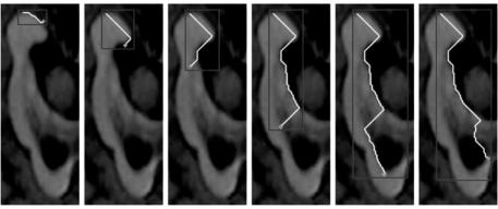
As can be seen in Fig. 14.10, the generated segmentation line approximates the edges present between the startand endpoint selected. The continuous computation of a global optimum leads to the jumping behavior of the algorithm, as can be observed in the last two images of Fig. 14.10. The last segment of the segmentation line abruptly changes the edges that are approximated.

Modifications of the resulting segmentation cannot be directly integrated in the concept of Live-Wires as the path array P is fixed solely based on the image on initialization, rendering any post processing a cumbersome task. To tackle the discontinuities, the user can generally fix the endpoint of the segmentation line so far if estimated adequately, thus freezing the wire and starting a new segment. A piecewise construction of the segmentation is obviously mandatory for any closed contour.

Different extensions have been proposed to improve the behavior of the LiveWire algorithms. These extensions include, but are not limited to the definition of more complex cost functions [38], advanced edge feature detections [40] and the extension to 3D [41–43]. The main advantages of the Live-Wire approach are the relatively simple implementation and the computational speed, as the

shortest path can be computed online while the user drags the mouse, thus providing direct feedback.

In contrast to Snakes, which will be described next, the selected path is a global optimum of the cost function defined over the complete image, whereas Snakes iteratively adapt their contours based on local information, which will very likely represent a local optimum of their respective target function. Global optimum is a desirable mathematical property in optimization; it is, however, not obvious that the best segmentation is equivalent to this definition of an optimum.

14.4.2 Snakes

The second class of algorithms presented intends to overcome some of the limitations of the graph-based approaches. The former allows the segmentation line, respectively surface, to have individual properties that are not related to the image, but rather to physical properties of some material. The segmentation process is no longer solely based on the image, but regularized by the constraineds imposed by the physical model. This model introduces some generic knowledge of general organ’s shape encoded in the elasticity of the material. The algorithms of this section belong to the field of physically based deformable models. In this section, the basics of Snakes are first depicted, followed by the presentation of two extensions that have been proposed during the last few years.

Traditional Snakes used for image segmentation are polygonal curves to which an objective function is associated. This function combines an “image term,” which measures either edge strength or edge proximity, and a regularization term, which accounts for tension and curvature. The curve is deformed in order to optimize a score and, as a result, to match the image edges. The optimization typically is global, i.e., it takes edge information into account along the whole curve simultaneously, but only considers local image information, i.e. image intensities close to the curve.

Snakes were originally introduced by Kass et al. [44] and are modeled as time-dependent 2-D curves defined parametrically as

where s is proportional to the arc length, t the current time, and x and y the curve’s image coordinates. The Snake deforms itself as time progresses so as to

minimize an energy term that combines image, internal, and external energies:

These energies are derived by integration along the curve. The forces resulting from the minimization of the image energy Eimage guide the Snake to match the desired image features. This image energy is derived by integrating over a potential P(v"(s, t)) from an image feature map, i.e.

1

Eimage(v) = − P(v(s, t)) ds (14.7)

0

A typical choice is to take P(v(s, t)) to be equal to the magnitude of the image gradient, that is

where I is either the image itself or the image convolved by a Gaussian kernel. As for the Live-Wire cost function, many different feature maps have been suggested in the past [45–47], yet the results are comparable.

The internal energy term Eint models the physical behavior of the material describing the Snake. Using the elastic rod model, Eint is taken to be

The parameters α(s) and β(s) are arbitrary functions that regulate the curve’s tension and rigidity and are commonly supplied by the user. It has been shown that they can be chosen in a fairly image-independent way [46]. Generally α(s) and β(s) are defined as constant along the curve, i.e. α(s) = α and β(s) = β. Other authors have proposed to dynamically adjust the values of α and β along the curve by a feed-back strategy [48].

The segmentation process performed with Snakes is governed by the min-

>

imization of the term E(v) dt. This amounts to using Hamilton’s principle in variational calculus to derive the Euler–Lagrange equations of motion. The resulting equation of motion for the basic Snake described here can be written as

γ (s) being the damping coefficient.

The segmentation process is now determined by the minimization of the

>

term E(v) + EK(v) + D(vt ) dt. Using the Hamiltonian principle the following Euler–Lagrange differential equation results

where µ(s) and γ (s) are considered constants along the curve. Forward differences are used to approximate the time derivatives, resulting in a linear system of equations which can be formulated in matrix notation as

((µ + γ )I + K) · v [t] = −Pv v[t−1] + (2µ + γ ) v [t−1] − µ v [t−2]. (14.16)

The role of the damping becomes evident, as the condition of the stiffness matrix

K is improved through the damping term (µ + γ )I. This term has to be selected in a reasonable manner to prevent the Snake to be “glued,” which would be the case for |(µ + γ )I| # |K|. With appropriate selections for µ and γ , a wellconditioned linear system results, so that the term (µ + γ )I + K can be inverted and Eq. (14.16) solved for v [t] yielding an iterative algorithm to solve the Snake equation of motion.

The Lagrangian formalism allows to unify forces from very different type of

sources. The target function is extended to incorporate more energy terms so

that the final energy to be minimized is of the form Etot = i Ei. Some basic extensions that have been presented are summarized.

14.4.2.3 External Forces

User interaction is introduced through external forces, so that the Snake can be modified manually [49]. Two type of forces are commonly used to attract or repulse the Snake from the current mouse position. Attraction can be modeled by introducing a virtual spring connecting the mouse position m with a point p on the Snake, that adds a term k(p − m)2 to the external energy Eext, where the spring constant k is a parameter. To push the Snake away from an undesired local energy minimum, a “volcano” is introduced by adding an energy function

proportional to r12 to the external energy, where r is the distance of a point from the volcano center. Obviously, special care is required to avoid instabilities near r = 0.

14.4.2.4 Balloon Forces

Traditional Snakes exhibit a tendency to shrink, as they reach an absolute minimum when contracted into a single point under a flat potential field, i.e., a homogeneous image. While the correction of the energy term Eint to enforce parameterization according to the arc-length can prevent this behavior, the resulting governing equations are highly nonlinear. Instead, an inflating force can be introduced, which expands a closed Snake like a balloon [50]. Denoting the unit vector normal to the curve at point v(s) with n(s), the additional energy term becomes

1

EB(v) = n(s) ds. (14.17)

0

14.4.2.5 Gravitational Forces

Similar to the balloon forces, a gravitational force can be defined [51]. Interpreting the image intensity as the z-dimension, the energy term is defined as

where g(s) is the gravitation vector (0, 0, −g). The Snake is then accelerated in negative z-direction, so that the model seems to “falls” on an object.

14.4.3 Deformable Surface Models

The basic concepts of Snakes—minimization of an energy term through optimization—can easily be generalized to three dimensions. Additional effort is required only to handle the parameterization problem adherent to 2-D manifolds.

In contrast to 2-D active contour models, where arc length provides a natural parameterization, 2-D manifolds as used for 3-D deformable models pose a complex, topology, and shape-dependent parameterization problem. Parameterizing

a surface effectively is difficult because there is no easy way to distribute the grid points evenly across the surface.

A generalized deformable surface model is defined as

where ω 2 is a suitable parameterization, t the current time, and x, y and z are the corresponding coordinate functions of the surface. Analogous to the 2D case, the surface deforms itself so as to minimize its image potential energy. Instead of the elastic rod model, the thin plate under tension model is employed to regulate the model’s shape during energy minimization. Thus, the

where ρ(ω) = 1 − τ (ω) for convenience and ω = (φ, θ ). The surface tension parameter τ is a user-supplied parameter in the range 0..1, varying the behavior of the surface between a thin plate (τ = 0) and a membrane (τ = 1). When endowing the surface with a mass µ and embedding it into a viscous medium the corresponding energy terms are the same as for the traditional Snake:

The Euler–Lagrange differential equation for constant parameters µ, γ , τ can be formulated

where v stands for either x, y, or z. These coupled differential equations can be solved numerically as in two dimensions.

14.4.4 Tamed Snakes

Despite their ability to approximate objects with little user input, the approaches reported so far lack an intuitive manipulation semantic. The primitive manipulation metaphors presented, spring and volcano, can only be applied directly on the Snake’s curve v. It would be desirable though to have a more powerful interaction method at hand, for example, to modify parts of the shape on a coarse