

Kluwer - Handbook of Biomedical Image Analysis Vol
.2.pdf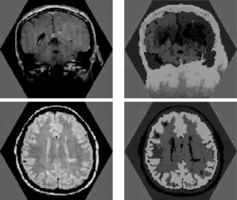
684 |
Herman and Carvalho |
Figure 12.8: Two images obtained using magnetic resonance imaging (MRI) of heads of patients (left) and the corresponding 3-segmentations (right). (Color slide.)
to be segmented, in the three objects being pairwise disjoint as well.) The right column of Fig. 12.8 shows the resulting maps of the σm by assigning the color
(r, g, b) = 255 × (σ1c, σ2c, σ3c) to the spel c. Note that not only the hue, but also the brightness of the color is important: the less brightly red areas for the last
two images correspond to the ventricular cavities in the brain, correctly reflecting a low grade of membership of these spels in the object that is defined by seed spels in brain tissue. The seed sets Vm consist of the brightest spels. The times taken to calculate these 3-segmentations using our algorithm on a 1.7 GHz Intel R XeonTM personal computer were between 90 and 100 ms for each of the seven images (average = 95.71 ms). Since these images contain 10,621 spels, the execution time is less than 10 s per spel. The same was true for all the other 2-D image segmentations that we tried, some of which are reported in what follows.
To show the generality of our algorithm and to permit comparisons with other algorithms, we also applied it to a selection of real images that appeared in the recent image segmentation literature. Since in all these images V consist of squares inside a rectangular region, the π of Eq. (12.2) is selected to
Simultaneous Fuzzy Segmentation of Medical Images |
685 |
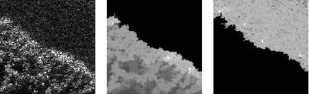
Figure 12.9: An SAR image of trees and grass (left) and its 2-segmentation (center and right).
be the edge-adjacency (4-adjacency) on the square grid. We chose to include in the sets of seed spels not only the spels at which the user points but also their eight edge-or-vertex adjacent spels. Except for this adaptation, the previous specification is verbatim what we use for the experiments which we now describe.
In [31] the authors demonstrate their proposed technique by segmenting an SAR image of trees and grass (their Fig. 1, our Fig. 12.9 left). They point out that “the accurate segmentation of such imagery is quite challenging and in particular cannot be accomplished using standard edge detection algorithms.” They validate this claim by demonstrating how the algorithm of [32] fails on this image. As illustrated on the middle and right images of Fig. 12.9, our technique produces a satisfactory segmentation. On this image, the computer time needed by our algorithm was 0.3 s (on the same 1.7 GHz Intel R XeonTM personal computer that we use for all experiments presented in this section), while according to a personal communication from the first author of [31], its method “took about 50 seconds to reach the 2-region segmentation for this 201-by-201 image on Sparc 20, with the code written in C.”
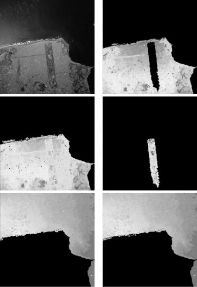
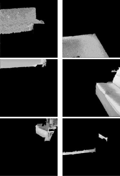
In Figs. 12.10–12.12 we report on the results of applying our approach to two physically obtained images from [6]: an aerial image of San Francisco (top-left image of Fig. 12.10) and an indoor image of a room (top-left image of Fig. 12.11). The middle and bottom images of the left column of Fig. 12.10 show a 2-segmentation of the San Francisco image into land and sea, while the right column shows how extra object definitions can be included in order to produce a more detailed labeling of a scene, with the 3-segmentation of the San Francisco image separating the Golden Gate Park from the rest of the land object. Figure 12.11 shows the original image (top-left) and a 5-segmentation of the
Simultaneous Fuzzy Segmentation of Medical Images |
687 |
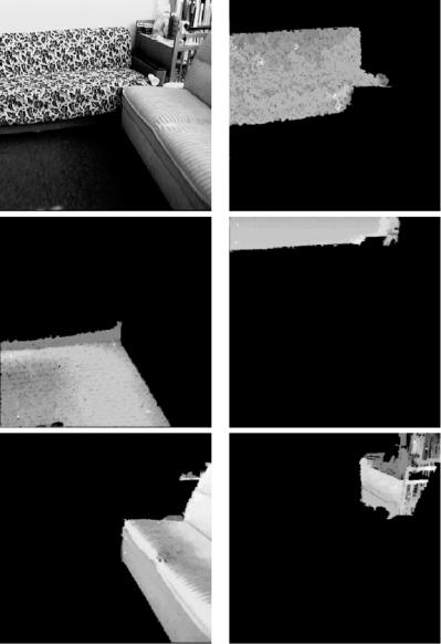
Figure 12.11: An indoor image of a living room (top left) and its 5-segmentation.
living room image. The 6-segmentation of the room shown in Fig. 12.12 includes a new object corresponding to the base and arm of one of the sofas.
It is stated in [6] that the times needed for the segmentations reported in that paper “are in the range of less than five seconds” (on a Sun UltraSparcTM ). Our CPU time to obtain the segmentations shown in Figs. 12.10–12.12 is
688 |
Herman and Carvalho |
Figure 12.12: A 6-segmentation of the indoor image of a living room shown in
Fig. 12.11.
around 2 s. However, there is a basic difference in the resolutions of the segmentations. Since the segmentation method used in [6] is texture based, the original 512 × 512 images are subdivided into 64 × 64 “sites” using a square window of size 8 × 8 per site. In the final segmentations of [6] all pixels in a particular
Simultaneous Fuzzy Segmentation of Medical Images |
689 |
window are assigned to the same object. As opposed to this, in our segmentations any pixel can be assigned to any object. Another way of putting this is that we could also make our spels to be the 8 × 8 windows of [6] and thereby reduce the size of the V to be a 64th of what it is currently. This should result in a two order of magnitude speedup in the performance of our segmentation algorithm (at the cost of a loss of resolution in the segmentations to the level used in [6]).
12.3.4 Accuracy and Robustness
Because all affinities (and consequently the segmentations) shown in the last section are based on seeds selected manually by a user, the practical usefulness and performance of the multiseeded fuzzy segmentation algorithm need to be experimentally evaluated, both for accuracy and for robustness.
The experiments used the top-left images of Figs. 12.3–12.7. We chose these images because they were based on mathematically defined objects to which we assigned gray values that were then corrupted by random noise and shading, and so the “correct” segmentations were known to us.
We then asked five users who were not familiar with the images to perform five series of segmentations, where each series consisted of the segmentation of each one of the five images presented in a random order. Since each of the five users performed five series of segmenting the five images, we had at our disposal 125 segmentations that were analyzed in a number of different ways.
First, we analyzed the segmentations concerning their accuracy. We used two reasonable ways of measuring the accuracy of the segmentations: in one we simply consider if the spel is assigned to the correct object, in the other we take into consideration the grade of membership as well. The point accuracy of a segmentation is defined as the number of spels correctly identified divided by the total number of spels multiplied by 100. The membership accuracy of a segmentation is defined as the sum of the grades of membership of all the spels which are correctly identified divided by the total sum of the grades of membership of all spels in the segmentation multiplied by 100.
The average and the standard deviation of the point accuracy for all 125 segmentations were 97.15 and 4.72, respectively, while the values for their membership accuracy were 97.70 and 3.82. These means and standard deviations are very similar. This is reassuring, since the definitions of both of the accuracies
690 |
Herman and Carvalho |
are somewhat ad hoc and so the fact that they yield similar results indicates that the reported figures of merit are not over-sensitive to the precise nature of the definition of accuracy. The slightly larger mean for the membership accuracy is due to the fact that misclassified spels tend to have smaller than average grade of membership values.
The average error (defined as “100 less point accuracy”) over all segmentations is less than 3%, comparing quite favorably with the state of the art: in [6] the authors report that a “mean segmentation error rate as low as 6.0 percent was obtained.”
The robustness of our procedure was defined based on the similarity of two segmentations. The point similarity of two segmentations is defined as the number of spels which are assigned to the same object in the two segmentations divided by the total number of spels multiplied by 100. The membership similarity of two segmentations is defined as the sum of the grades of memberships (in both segmentations) of all the spels which are assigned to the same object in the two segmentations divided by the total sum of the grades of membership (in both segmentations) of all the spels multiplied by 100. (For both these measures of similarity, identical segmentations will be given the value 100 and two segmentations in which every spel is assigned to a different object will be given the value 0.)
Since each user segmented each image five times, there are 10 possible ways of pairing these segmentations, so we had 50 pairs of segmentations per user and a total of 250 pairs of segmentations. Because the results for point and membership similarity were so similar for every user and image (for detailed information, see [29]) we decided to use only one of them, the point similarity, as our intrauser consistency measure. The results are quite satisfactory, with an average intra-user consistency of 96.88 and a 5.56 standard deviation.
In order to report on the consistency between users (interuser consistency) we selected, for each user and each image, the most typical segmentation by that user of that image. This is defined as that segmentation for which the sum of membership similarities between it and the other four segmentations by that user of that image is maximal. Thus, we obtained five segmentations for each image that were paired between them into 10 pairs, resulting into a total of 50 pairs of segmentations. The average and standard deviation of the interuser consistency (98.71 and 1.55, respectively) were even better than the intrauser
Simultaneous Fuzzy Segmentation of Medical Images |
691 |
consistency, mainly because the selection of the most typical segmentation for each user eliminated the influence of relatively bad segmentations.
Finally, we did some calculations of the sensitivity of our approach to M
(the predetermined number of objects in the image). The distinction between the objects represented in the top right and bottom left images of Fig. 12.5 and between the objects represented in the bottom images of Fig. 12.7 is artificial; the nature of the regions assigned to these objects is the same. The question arises: if we merge these two objects into one do we get a similar 2-segmentation to what would be obtained by merging the seed points associated with the two objects into a single set of seed points and then applying our algorithm? (This is clearly a desirable robustness property of our approach.) The average and standard deviation of the point similarity under object merging for a total of 50 readings by our five users on the top-left images of Figs. 12.5 and 12.7 were 99.33 and 1.52, respectively.
12.4 3-D Segmentation
As showed before, the multiseeded segmentation algorithm is general enough to be applied to images defined on various grids. One has several options for representing a 3D image; in this section, when performing segmentation on 3D images, we choose to represent them on the face-centered cubic (fcc) grid, for reasons that are presented later.
Using Z for the set of all integers and δ for a positive real number, we can define the simple cubic (sc) grid (Sδ ), the face-centered cubic (fcc) grid (Fδ ) and the body-centered cubic (bcc) grid (Bδ ) as
Sδ = {(δc1, δc2, δc3) | c1, c2, c3 Z} , |
(12.16) |
|
Fδ = {(δc1, δc2, δc3) | c1 |
, c2, c3 Z and c1 + c2 + c3 ≡ 0 (mod 2)} , |
(12.17) |
Bδ = {(δc1, δc2, δc3) |
| c1, c2, c3 Z and c1 ≡ c2 ≡ c3 (mod 2)} , |
(12.18) |
where δ denotes the grid spacing. From the definitions above, the fcc and bcc grids can be seen either as one sc grid without some of its grid points or as a union of shifted sc grids, four in the case of the fcc and two in the case of the bcc.
We now generalize the notion of a voxel to an arbitrary grid. Let G be any set of points in R3, then the Voronoi neighborhood of an element g of G is
692 |
Herman and Carvalho |
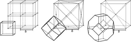
Figure 12.13: Three grids with the Voronoi neighborhood of one of their grid points. From left to right: the simple cubic (sc) grid, the face-centered cubic (fcc) grid, and the body-centered cubic (bcc) grid.
defined as |
|
NG (g) = {v R3 | for all h G, v − g ≤ v − h}. |
(12.19) |
In Fig. 12.13, we can see the sc, the fcc and the bcc grids and the Voronoi neighborhoods of the front-lower-left grid points.
Why should one choose grids other than the ubiquitous simple cubic grid? The fcc and bcc grids are superior to the sc grid because they sample the 3-D space more efficiently, with the bcc being the most efficient of the three. This means that both the bcc and the fcc grid can represent a 3-D image with the same accuracy as that of the sc grid but using fewer grid points [33].
We decided to use the fcc grid for 3-D images instead of the bcc grid for reasons that will become clear in a moment; now we discuss one additional advantage of using the fcc grid over the sc grid. If we have an object that is a union of Voronoi neighborhoods of the fcc grid, then for any two faces on the boundary between this object and the background that share an edge, the normals of these faces make an angle of 60◦ with each other. This results in a less blocky image than if we used a surface based on the cubic grid with voxels of the same size. This can be seen in Fig. 12.14, where we display approximations to a sphere based on different grids. Note that the display based on the fcc grid (center) has a better representation than the one based on the sc grid with the same voxel volume (left) and is comparable with the representation based on cubic grid with voxel volume equal to one eighth of the fcc voxel volume (right).
The main advantage of the bcc grid over the fcc grid is that it needs fewer grid points to represent an image with the same accuracy. However, in the bcc