Kluwer - Handbook of Biomedical Image Analysis Vol

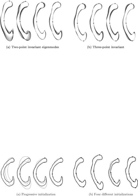
Figure 14.14: The first five one-point invariant eigenmodes after the subtraction

of the first principal landmark. The various shapes are obtained by evaluating

ˆ ˆ

p + ω λkj ukj with ω {−2, . . . , 2} and k {1, . . . , 5}.

ˆ

Doing so for all instances, we obtain a new description of our population bij which is invariant with respect to point j. An example of the removal of the variation is visualized in Fig. 14.14.

In order to further improve the point-wise elimination process, the control point selection strategy has to be optimized. This can be done by choosing control vertices, or principal landmarks, which carry as much shape information as possible.

We define the reduction potential of a vertex jk being a candidate to serve as the kth principal landmark by

principal landmarks that have been removed from the statistic in the given order, and the superscript ◦sˆk indicating the value of ◦ if the principal landmarks sˆk have been removed.

In order to remove as much variation as possible, we choose consequently that point as the first principal landmark that holds the largest reduction

eigenmodes shown in Fig. 14.14. Further application of the selection strategy

selecting three to four landmarks has proven to be sufficient for a reasonably good initialization.

14.6 Improving Human–Computer Interaction

14.6.1 Background

Extensive research has been invested in recent years into improving interactive segmentation algorithms. It is, however, striking that the human–computer interface, a substantial part of an interactive setup, is usually not investigated. Although the need for understanding the influence of human–computer interaction on interactive segmentation is recognized, only very little research has been done in this direction.

In order to improve information flow and to achieve optimal cooperation between interactive image analysis algorithms and human operators, we evaluated closed-loop systems utilizing new man–machine interfacing paradigms [62].

The mouse-based, manual initialization of deformable models in two dimensions represents a major bottleneck in interactive segmentation. In order to overcome the limitations of 2-D viewing and interaction the usage of direct 3-D interaction is inevitable. However, adding another dimension to user interaction causes several problems. Editing, controlling, and interacting in three dimensions often overwhelms the perceptual powers of a human operator. Furthermore, today’s desktop metaphors are based on 2-D interaction and cannot easily be extended to the volumetric case. Finally, the visual channel of the human sensory system is not suitable for the perception of volumetric data.

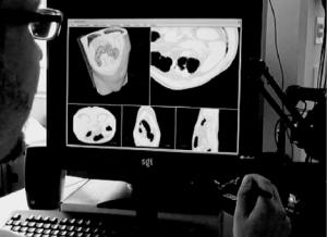
However, these major drawbacks are valid only in terms of interactive systems that are based on 2-D Window–Icon–Mouse–Pointer (WIMP) interfaces that solely rely on the visual sense of the human operator. In order to alleviate the limitations of visual-only systems we may try to enhance the interaction process with additional sensory feedback. The fundamental challenge here is to find efficient ways for information flow between user and computer. Several sensory channels could be addressed, but due to the 3-D nature of the problem, the most obvious choice is the haptic channel. As an example, a multimodal system using visual and haptic volumetric rendering will be described, which was successfully applied to the segmentation of the intestinal system (Fig. 14.17).

Figure 14.17: Interactive, multimodal setup.

14.6.2 Multimodal Segmentation

The validity of the multimodal approach is evaluated on the basis of the highly complex task of segmentation of the small intestine. Currently, no satisfying solutions exist to deal with this problem. Although the small intestine has a complex spatial structure, from a topological point of view it is a rather simple linear tube with exactly defined startand endpoint. Therefore, the key to solving the segmentation problem is to make use of the topological causality of the structure. The overall extraction process has to be mapped onto the linear structure of the intestinal system to simplify the task.

The initial step of our multimodal technique is the haptically assisted extraction of the centerline of the tubular structures. The underlying idea is to create guiding force maps, similar to the notion of virtual fixtures found in teleoperation [63, 64]. These forces can be used to assist a user’s movement through the complex dataset.

To do this we first create a binarization of our data volume V by thresholding. The threshold is chosen dependent on the grayscale histogram, but can also be specified manually. We have to emphasize that this step is not sufficient for a complete segmentation of the datasets we are interested in. This is due to the often low quality of the image data. Nevertheless, in the initial step we are not interested in a topologically correct extraction. On the contrary, we only need a rough approximation of our object of interest. From the resulting dataset W

for each (x, y, z) W , where d denotes the Euclidean distance from a voxel that is part of the tubular structure to a voxel of the surrounding tissue W = V \ W .

In the next step we negate the 3-D distance map and approximate the gradients by central differences. Moreover, to ensure the smoothness of the computed forces, we apply a 5 × 5 × 5 binomial filter. This force map is precomputed before the actual interaction to ensure a stable force-update. Because the obtained forces are located at discrete voxel positions, we have to do a trilinear interpolation to obtain the continuous gradient force map needed for stable haptic interaction. Furthermore, we apply a low-pass filter in time to further suppress instabilities. The computed forces can now be utilized to guide a user on a path close to the centerline of the tubular structure. In the optimal case of good data quality, the user falls through the dataset guided along the 3-D ridge created by the forces. However, if the 3-D ridge does not exactly follow the centerline the user can guide the 3-D cursor by exerting a gentle force on the haptic device to leave the precalculated curve.

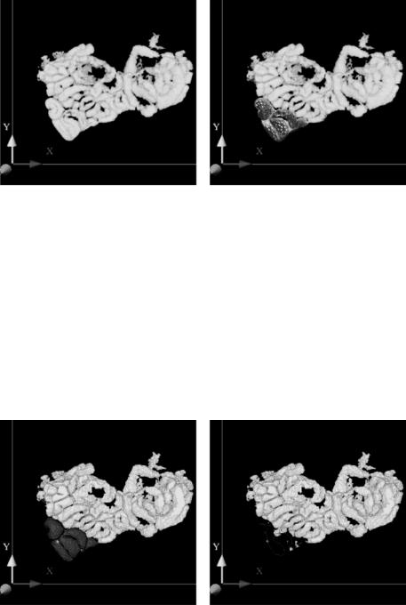
While moving along the path, points near the centerline are set. These points can be used to obtain a B-spline, which approximates the path. In the next step this extracted centerline is used to generate a good initialization for a deformable surface model. To do this, a tube with varying thickness is created according to the precomputed distance map. This resulting object is then deformed subject to a thin plate under tension model. Details of the algorithmic background of this deformable model approach are described in section 14.4.2.

Because of the good initialization, only a few steps are needed to approximate the desired object [65]. The path initialization can be seen in Fig. 14.18(a). Note, that the 3-D data is rendered semitransparent to visualize the path in the lower left portion of the data. Figure 14.18(b) depicts the surface model during deformation.

In order to further improve the interaction with complicated datasets a step- by-step segmentation approach can be adopted by hiding already segmented loops. This allows a user to focus attention on the parts that still have to be extracted. For this purpose the 3-D surface model is turned back into voxels and removed from the dataset (Fig. 14.19). This step can be carried out in

virtual fly-throughs. Further evaluation studies were performed, which show a statistically significant performance improvement in the trial time when using haptically enhanced interaction in 3-D segmentation. Also in the haptic condition the quality of segmentation was always superior to the one without force feedback.

14.7 Conclusions

In spite of the enormous research and development effort invested into finding satisfactory solutions during the past decades, the problem of medical image segmentation (as image segmentation in general) is still an unsolved problem today, and no single approach is able to successfully address the whole range of possible clinical problems. The basic reason for this rather disappointing status lies in the difficulties in representing and using the prior information in its full extent, which is necessary to successfully solve the underlying task in scene analysis and image interpretation.

While first results already clearly demonstrate the power of the model-based techniques, generic segmentation systems capable to analyze a broad range of radiological data even under severely pathological conditions cannot be expected in the near future. Currently available methods, like those discussed in this chapter, allow to work only within a very narrow, specialized problem domain and fundamental difficulties have to be expected if trying to establish more generic platforms. The practically justifiable number of examples in the training sets can cover only very limited variations of the anatomy and are usually applied to analyzing images without large pathological changes. It still needs a long way to go, before the computer representation and usage of the prior knowledge involved in the interpretation of radiological images can be represented and used by a computer in complexity which is sufficient to reasonably imitate the everyday work of an experienced clinical radiologist. Accordingly, in the near future only a well-balanced cooperation between computerized image analysis methods and a human operator will be able to efficiently address many clinically relevant segmentation problems. Better understanding of the perceptional and technical principles of man–machine interaction is therefore a fundamentally important research area which should now get significantly more attention than what it was getting in the past.

Bibliography

[1]Gerig, G., Martin, J., Kikinis, R., Kubler,¨ O., Shenton, M., and Jolesz, F., Automatic segmentation of dual-echo MR head data, In: Proceedings of Information Processing in Medical Imaging’91, Wye, GB, 1991, pp. 175–187.

[2]Duda, R. and Hart, P., Pattern Classification and Scene Analysis, Wiley, New York, 1973.

[3]Shattuck, D., Sandor-Leahy, S., Schaper, K., Rottenberg, D., and Leahy, R., Magnetic resonance image tissue classification using a partial volume model, Neuroimage, Vol. 13, pp. 856–876, 2001.

[4]S. Ruan, J. X., C. Jaggi and Bloyet, J., Brain tissue classification of magnetic resonance images using partial volume modeling, IEEE Trans. Med. Imaging, Vol. 19, No. 12, pp. 172–186, 2000.

[5]Gerig, G., Kubler,¨ O., Kikinis, R., and Jolesz, F., Nonlinear anisotropic filtering of MRI data, IEEE Trans. Med. Imaging, Vol. 11, No. 2, pp. 221– 232, 1992.

[6]Guillemaud, R. and Brady, M., Estimating the bias field of MR images, IEEE Trans. Med. Imaging, Vol. 16, No. 3, pp. 238–251, 1997.

[7]M. Styner, G. S., Ch. Brechbuhler¨ and Gerig, G., Parametric estimate of intensity inhomogeneities applied to MRI, IEEE Trans. Med. Imaging, Vol. 19, No. 3, pp. 153–165, 2000.

[8]Wells, W., Grimson, W., Kikinis, R., and Jolesz, F., Adaptive segmentation of MRI data, IEEE Trans. Med. Imaging, Vol. 15, No. 4, pp. 429–443, 1996.

[9]Van Leemput, K., Maes, F., Bello, F., Vandermeulen, D., Colchester, A., and Suetens, P., Automated segmentation of MS lesions from multichannel MR images, In: Proceedings of Second International Conference on Medical Image Computing and Computer-Assisted Interventions, MICCAI’99, Taylor, C. and Colchester, A., eds., Lecture Notes in Computer Science, Vol. 1679, Springer-Verlag, New-York, pp. 11–21, 1999.

[10]Li, S. Z., Markov Random Field Modeling in Computer Vision, SpringerVerlag, Tokyo, 1995.

[11]Serra, J., Image Analysis and Mathematical Morphology, Academic Press, San Diego, 1982.

[12]Raya, S., Low-level segmentation of 3-D magnetic resonance brain images—A rule-based system, IEEE Trans. Med. Imaging, Vol. 9, No. 3, pp. 327–337, 1990.

[13]Stansfield, S., ANGY: A rule-based system for automatic segmentation of coronary vessels from digital subtracted angiograms, IEEE Trans. Patt. Anal. Mach. Intell., Vol. 8, No. 2, pp. 188–199, 1986.

[14]Bajcsy, R. and Kovacic, S., Multiresolution elastic matching, Comput. Vision Graph. Image Process., Vol. 46, pp. 1–21, 1989.

[15]Evans, A. C., Collins, D. L., and Holmes, C. J., Toward a probabilistic atlas of human neuroanatomy, In: Brain Mapping: The Methods, Mazziotta, J. C. and Toga, A. W., eds., Academic Press ISBN 0126930198 pp. 343– 361, 1996.

[16]Jiang, H., Holton, K., and Robb, R., Image registration of multimodality 3-D medical images by chamfer matching, In: Proceedings of Biomedical. Image Processing and 3D Microscopy, SPIE, Vol. 1660, SPIE, The International Society of Optical Engineering pp. 356–366, 1992.

[17]Christensen, G., Miller, M., and Vannier, M., Individualizing neuroanatomical atlases using a massively parallel computer, IEEE Computer, pp. 32–38, January 1996.

[18]Bookstein, F., Shape and the information in medical images: A decade of the morphometric synthesis, Comput. Vision. Image Understand., Vol. 66, No. 2, pp. 97–118, 1997.

[19]Evans, A., Kamber, M., Collins, D., and MacDonald, D., An MRI-based probabilistic atlas of neuroanatomy, In: Magnetic Resonance Scanning and Epilepsy, Shorvon, S., ed., Plenum Press, New York, pp. 263–274, 1994.

[20]Wang, Y. and Staib, L., Elastic model based non-rigid registration incorporating statistical shape information, In: Proc. First Int. Conf. on Medical Image Comp. and Comp. Assisted Interventions, Vol. 1679 of Lecture Notes in Comp. Sci., pp. 1162–1173, Springer-Verlag, New York, 1998.

[21]Terzopoulos, D. and Metaxas, D., Dynamic 3D models with local and global deformations: Deformable superquadrics, IEEE Trans. Pattern Anal. Mach. Intell., Vol. 13, No. 7, pp. 703–714, 1991.

[22]Vemuri, B. and Radisavljevic, A., Multiresolution stochastic hybrid shape models with fractal priors, ACM Trans. Graphics, Vol. 13, No. 2,

pp.177–200, 1994.

[23]Staib, L. and Duncan, J., Boundary finding with parametrically deformable models, IEEE Trans. Pattern Anal. Mach. Intell., Vol. 14, No. 11,

pp.1061–1075, 1992.

[24]Brechbuhler,¨ C., Gerig, G., and Kubler,¨ O., Parametrization of closed surfaces for 3-D shape description, CVGIP: Image Understand., Vol. 61,

pp.154–170, 1995.

[25]Cootes, T., Cooper, D., Taylor, C., and Graham, J., Training models of shape from sets of examples, In: Proceedings of The British Machine Vision Conference (BMVC) Springer-Verlag, New-York, pp. 9–18, 1992.

[26]Cootes, T. and Taylor, C., Active shape models—‘Smart snakes,’ In: Proceedings of The British Machine Vision Conference (BMVC) SpringerVerlag, New-York, pp. 266–275, 1992.

[27]Rangarajan, A., Chui, H., and Bookstein, F., The softassign procrustes matching algorithm, information processing in medical imaging,

pp.29–42, 1997. Available at http://noodle.med.yale.edu/anand/ps/ ipsprfnl.ps.gz.

[28]Tagare, H., Non-rigid curve correspondence for estimating heart motion, Inform. Process. Med. Imaging, Vol. 1230, pp. 489–494, 1997.