Kluwer - Handbook of Biomedical Image Analysis Vol

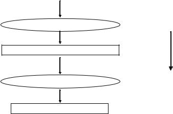
Assign One “Level Value” to Selected Class (es)

Left and Right Lumen Detected

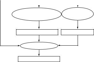
Figure 9.23: Region detection: region merging algorithm. The input image has lumens that have 1, 2, or more classes. If the number of classes in the ROI is one class, then that class is selected; if two classes are in the ROI, then the minimum class is selected; and if there are three or more classes in the ROI, then the minimum two classes are selected. The selected classes are merged by assigning all the pixels of the selected classes one level value. This process results in the left and right lumen being binarized.

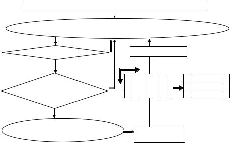
Lumen binary regions detected (2 lumens here)

Top to Down Labeling

R C

Top Down Labeling

Left to Right Labeling

Left Right Labeling

Figure 9.24: Region identification using connected component analysis (CCA). Input is an image in which the lumen binary regions are detected. The CCA first labels the image from the top to the bottom, and then from the left to the right. The result is an image that is labeled from the left to the right.

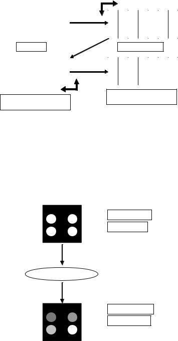
Figure 9.25: Region identification: ID assignment. In the connected component analysis (CCA), in the input binary image each white pixel is assigned a unique ID. Then the label propagation process results in connected components.

the region from left to right is shown in Fig. 9.26. This is the first pass of the labelpropagation process. Every row of the image is scanned from top to bottom, left to right, pixel by pixel. If the pixel has an ID, then pixels to the left and above of the pixel are checked for IDs, and if either one has an ID, then the pixel’s value is reassigned to that of the lowest among the neigbor pixels and the pixel. This processed is repeated for all pixels in the row and in all rows. The result is a binary image with some label propagation. The propagation of the region from top to bottom is shown in Fig. 9.27. This is the second pass of the labelpropagation process. Every row of the image is scanned from bottom to top, right to left, pixel by pixel. If the pixel has an ID, then pixels to the right and below of the pixel are checked for IDs, and if either one has an ID, then the pixel’s value is reassigned to that of the lowest among the neigbor pixels and the pixel. This processed is repeated for all pixels in the row and in all rows. The result is a binary image with some label propagation. Finally, the region assignment is summarized in Fig. 9.28. The top left image is a binary image with a value of 1 assigned to each of the white pixels. Each of the white pixels are assigned a unique value in the top-right image. The left to right and top to bottom label propagation propagates the labels of value 1 and 3, and the result is the

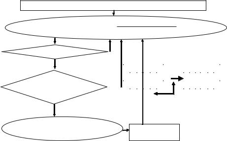
Binary Image: Each white pixel has unique ID

For each row of the image, scan (bottom to top, right to left) each pixel

NO

Does pixel have an ID?

Re-assign pixel lowest of neighbor

IDs and pixel ID

Binary Image:

Reassigned Pixel

Figure 9.27: Region identification: propagation. This is the second pass of the label propagation process. Given the binary image having unique IDs for each white pixel, every row of the image is scanned from bottom to top, right to left, pixel by pixel. If the pixel has an ID, then pixels to the right and below of the pixel are checked for IDs, and if either one has an ID, then the pixel’s value is reassigned to that of the lowest among the neigbor pixels and the pixel. This processed is repeated for all pixels in the row and all rows. The result is a binary image with reassigned pixel values.

in green estimated boundary image. These three images are fused to produce a color overlay image.

9.4.4 Results of Synthetic System: Boundary Estimation

Figure 9.31 shows in the FCM classification system all the steps for the left and right lumen detection, identification, and boundary estimation process in the synthetic images. We look at large noise protocol as an example below with noise level σ 2 = 500. In the first row the left image shows the synthetically generated image. In the first row the right image shows the image after it has been smoothed by the Perona–Malik smoothing function. In the second row the left image shows the classified image after the image has gone through the FCM

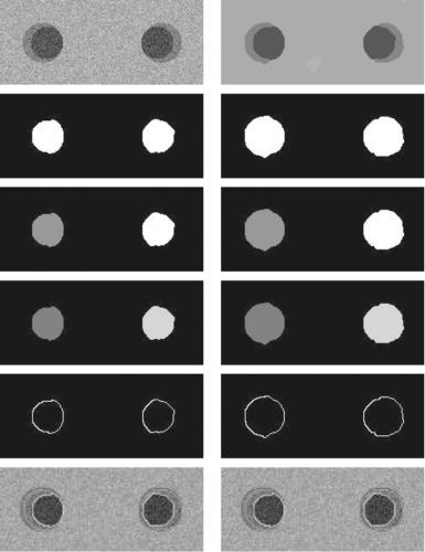
noise level σ 2 = 500. In the first row the left image shows the synthetically generated image. In the first row the right image shows the classified image after the image has gone through the MRF classification system. In the second row the left image shows the binarization of the image after selecting only the core class for binarization (K = 1). In the second row the right image shows the binarization of the image after selecting the core class and the edge classes for binarization (K > 1). In the third row the left image shows the image (K = 1) after the labeling of CCA. In the third row the right image shows the image (K > 1) after the labeling of CCA. In the fourth row the left image shows the image (K = 1) after the labeling of assign ID. In the fourth row the right image shows the image (K > 1) after the labeling of assign ID. In the fifth row the left image shows the computer-estimated boundary of the image (K = 1), using the region-to-boundary algorithm. In the fifth row the right image shows the computer-estimated boundary of the image (K > 1), using the region-to- boundary algorithm. In the sixth row the left image shows the original image on which is overlayed the ideal ground truth boundary, the artifacted boundary (K = 1), and the corrected boundary (K > 1). In the sixth row the right image shows the original image on which is overlayed the ideal ground truth boundary, the artifacted boundary (K = 1), and the corrected boundary (K > 1).

Figures 9.33 and 9.34 show in the GSM classification system all the steps for the left and right lumen detection, identification, and boundary estimation process in the synthetic images. We look at large noise protocol as an example below with noise level σ 2 = 500. In Fig. 9.33, the first row the left image shows the synthetically generated image. In the first row the right image shows the image after it has been smoothed by the Perona–Malik smoothing function. In the second row the left image shows the image after its frequency peaks of pixel values have been merged. In the second row the right image shows the classified image after the image has gone through the GSM classification system. In the third row the left image shows the binarization of the image after selecting only the core class for binarization (K = 1). In the third row the right image shows the binarization of the image after selecting the core class and the edge classes for binarization (K > 1). In the fourth row the left image shows the image (K = 1) after the labeling of CCA. In the fourth row the right image shows the image (K > 1) after the labeling of CCA. In Fig. 9.34, the first row the left image shows the image (K = 1) after the labeling of assign ID. In the first row the right image shows the image (K > 1) after the labeling of assign

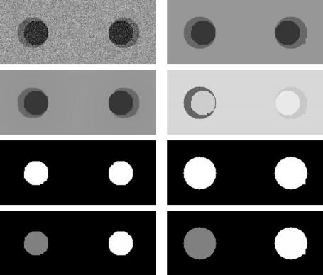
Figure 9.33: Results on synthetic image with noise variance, σ 2 = 500 using GSM method. Row 1, left: Synthetic generate image. Row 1, right: After peak merger. Row 2, left: After Perona–Malik Smoothing. Row 2, right: After GSM classification system. Row 3, left: Binarization with only C0 class (K = 1). Row 3, right: Binarization with merging C0, C1, and C2 classes (K > 1). Row 4, left: Binarization after CCA (K = 1). Row 4, right: Binarization after CCA (K > 1).

ID. In the second row the left image shows the computer-estimated boundary of the image (K = 1), using the region-to-boundary algorithm. In the second row the right image shows the computer-estimated boundary of the image (K > 1), using the region-to-boundary algorithm. In the third row the left image shows the original image on which is overlayed the ideal ground truth boundary, the artifacted boundary (K = 1), and the corrected boundary (K > 1). In the third row the right image shows the original image on which is overlayed the ideal ground truth boundary, the artifacted boundary (K = 1), and the corrected boundary (K > 1).