Kluwer - Handbook of Biomedical Image Analysis Vol

where k is the iteration cycle and τ is the constant. Even though this schedule can guarantee a global minimum solution, unfortunately, it is normally too slow for practical applications. Some other annealing methods [58] have been proposed to reduce the computation burden; unfortunately, it is no longer guaranteed to reach global minimum.

8.2.2.3.2 Iterated Conditional Modes. The goal of the ICM algorithm, proposed by Besag [33] in 1974, is to find a numerical approximation to further reduce the amount of computation produced by using stochastic relaxation. In recent publications, Pappas introduced an adaptive method [20] based on ICM and Chang et al. [46] extended it to color image segmentation.

In ICM algorithm, two assumptions are applied to the Markov random field:

(i)Given random field X, the observation components, Yi, are modeled as the independent and identical distributed (i.i.d.) white Gaussian noise, with zero mean and variance s2, and they are with the same known conditional density function p(Ys | Xs), dependent only on Xs. The conditional probability can be expressed as

(ii)The labeling of pixel s, Xs, depends only on the labels of its local neighborhood as

This is actually the Markovian property.

Under these assumptions, the conditional a posterior probability can be written as

where Ns is the neighborhood of pixel s and Cs is the set containing all the cliques

within Ns. This equation shows that the local conditional probability depends only on Xs, Ys, and Ns.

Based on these relations, the ICM iteratively decreases the energy by visiting and updating the pixels in a raster-scan order. For each pixel s, given the observed image Y and the current label of all the other pixels (actually only the neighborhood of pixel s), the label of Xs is replaced with one that can maximize

Starting from the initial state, this algorithm will keep on running based on the procedure introduced above until either the predefined number of iterations is reached or when the labels of X do not change any more. Then it is regarded that a local minimum is reached.

Compared with the acceptance probability in SA method, only decrease of energy change is accepted in the ICM algorithm. This can be regarded as a spatial case when T = 0 because SA never accept any positive energy change when T is at zero temperature. This is why ICM is often referred as the “instant freezing” case of simulated annealing.

Even though ICM provides a much faster convergence than stochastic relaxation based methods, the solutions from ICM are likely to reach only local minima and there is no guarantee that a global minimum of energy function can be obtained. Also, the initial state and the pixel visiting sequence can also have effects on the searching result.

8.2.2.3.3 Highest Confidence First. Highest confidence first (HCF) algorithm, proposed by Chou and Brown [21], is another deterministic method for combinatorial minimization. Similar to the ICM algorithm, the two assumptions in Eqs. (8.19)–(8.21) also hold for HCF, and the minimal energy estimation, equivalent to maximizing the conditional a posterior probability of p(Xs | Y, Xr , all r = s) for each pixel s, is also implemented iteratively.

The core feature of the HCF algorithm is the design of sites’ label updating scheme. Assume L, with size NL , is the set of the labels that are assigned to each site in the segmentation label matrix, which includes a special label 0 L to indicate the initial state of all sites. In the HCF algorithm, the site labeled with 0 is called “uncommitted site”; otherwise, it is called “committed site.”

384 Xu et al.

In the optimization process, once a label is assigned to an uncommitted site, the site becomes committed and cannot return to uncommitted state any more. However, a committed site can update its label through another assignment.

Instead of considering the energy change on an individual site through a raster-scan sequence as that in ICM, the HCF algorithm has the energy changes on all sites of the image within consideration via a measurement, called confidence, and updates the one with the highest confidence. The definition of confidence is derived from the local conditional probability in Eq. (8.22). Assume

where l L , is the segmentation label. The confidence measure cs(x) at site s is defined as

(8.26)

In Eq. (8.26), Lmin is the one that can make the energy function at site s minimum among all the elements except 0 in label set L. When a site is uncommitted, it is obvious that cs(x) is always nonnegative. Label of the site with the maximum amount of confidence will be changed to Lmin. The exact purpose of this label updating process is to actually pick up the site where an appropriate label assignment can lower the energy of the whole image the most. In the meantime, the new label of this site influences the energy and confidence of its neighbors whose confidences need to be updated before the start of the next iteration. We can also regard the confidence as an indication that how stable the segmentation will be with the changing of the label at s. Obviously, the more stable is the label-updated image due to the change, the more confident we are that the label at s should be updated.

The HCF algorithm initially assigns all the sites with label 0 in the segmentation matrix. In each iteration, the algorithm will update only the site with the maximum confidence to the label that minimizes Es the most. In the calculation of cs(x), only neighbors that are committed can affect the clique potentials. Therefore, once the label of a site changes, either from uncommitted state to committed state or from one committed label to another committed label, the confidence of its neighbors will have to be recalculated. The HCF algorithm stops when all the sites are committed and their confidence becomes negative.

Although it is claimed [46] that there is no initial estimate needed in HCF, some parameters, such as the mean value of each site, have to be provided in advance in order to get the confidence calculated when all the sites are uncommitted. For implementation, a heap structure is suggested in Chou’s design that creates the highest confidence in the searching process faster.

Even though both the ICM and the HCF algorithms can only reach local minima of energy function, the results obtained with HCF are generally better than that with ICM [19, 46] because of its relatively optimal label-updating scheme. In HCF, the optimization result is independent of the scanning order of the sites. Even though this may lead to the increase of the computation amount and implementation complexity, the HCF algorithm is still regarded as a very practical solution with the fast growing of the processors’ power.

8.2.3 QHCF Method

8.2.3.1 Algorithm

In the optimization procedure of the original HCF algorithm proposed by Chou and Brown [21], all the pixels are uncommitted and labeled 0 at the very beginning. A (prechosen) number of classes K are required in advance and the whole image is then presegmented (usually by K -means clustering) into K regions. The purpose is to estimate the mean of region that each pixel belongs to so as to initialize the energy of the whole image for HCF updating, and as the segmentation result is very sensitive to this initialization, the choice of K becomes very critical.

To overcome this problem, in the proposed QHCF algorithm, we first apply a Quad-Tree procedure to presegment the image instead of using K -means. The

advantages are as follows:

(i)There is no need to predefine the number of classes because the QuadTree algorithm can dynamically decide the partitions based on its splitting criterion.

(ii)K -means is a clustering method, in which the grouping is done in the measurement domain and has no spatial connectivity constraint to those pixels with the same label during the iteration process, while in the QuadTree splitting process, the grouping of pixels is done in the image spatial domain so that each region will not share labels with others.

The Quad-Tree procedure initially divides the whole image into four equalsize blocks. By checking the value of region criterion (RC) Vrc, each block will be evaluated whether it is qualified to be an individual region. The RC for each block Bi is defined as

If Vrc is smaller than a predefined threshold Trc, the block is regarded as a region. Otherwise, it will further be divided into smaller blocks by the same splitting method until every small block satisfies. The choice of Trc is applicationdependent and defines how uniform each region will be.

Compared with the other systematic initialization schemes, such as uniform grid initialization presented in [19], the Quad-Tree initialization is more accurate and efficient in adaptive detection of the initial regions. The reasons are listed as follows:

(i)The selection of initial sites is based on the consideration of pixels in the surrounding region due to the spatial constraint.

(ii)The points within the same region are not used for initialization repeatedly so that unnecessary computations can be avoided.

(iii)The iterative comparisons can be simplified during the HCF labeling process and the problem of “unlabeled small region” in [19] can be solved.

Moreover, by applying the Quad-Tree preestimation, the segmentation result can be more consistent than the uniform grid method when the initialization parameter changes in certain situations (this will be shown by experimental results at the end of this section).

Use Quad-Tree to pre-partition image into m regions

Label the prototype

Quad-Tree block

Yes

Any pixel has negative confidence?

No

Select the pixel with highest confidence, and label it to get minimum energy

Update energy & confidence

End of segmentation

Figure 8.3: Procedures of the QHCF algorithm.

After the Quad-Tree initialization, in each region, the pixel with closest value to the mean of region intensity is selected as the representative and assigned a unique label; the others are all uncommitted and labeled 0. The algorithm will then start to update labels according to the procedures given in Fig. 8.3 until the energy of the whole image becomes stable. In this label updating process, the pixels are permitted to change only within the committed states or from uncommitted states to committed states. They are not allowed to become uncommitted from committed states.

To simplify the calculation, we assume variance with σ 2 = 12 . The local energy is normalized as

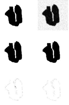
Figure 8.4: A phantom study of the MRF segmentation problem with adaptive ICM and QHCF. (a) Original phantom image. (b) Phantom is processed with additive Gaussian random noise. (c) Segmented image with Pappas’ adaptive ICM algorithm. (d) Segmented result with proposed QHCF algorithm. (e) The difference between (a) and (c). Number of dark pixels is 120. (f) The difference image between (a) and (d). Number of dark pixels is 92.

accuracy. In this study, a phantom was used as the ground truth shown in Fig. 8.4(a). By applying additive Gaussian noise, a test image was created as shown in Fig. 8.4(b). It was segmented with adaptive ICM [20] and the QHCF algorithms individually. The results are shown in Figs. 8.4(c) and 8.4(d). Comparison of the segmented images with the original phantom images yielded difference images (Figs. 8.4(e) and 8.4(f)). QHCF had 92 pixel errors, while adaptive ICM had 120 pixel errors. Ten phantom image comparisons had been conducted and the QHFC algorithm sustained 24.7% fewer edge pixel errors than the ICM algorithm. We can also see from the shape of the ICM-segmented object that

merging of the two parts has occurred, while the proposed QHFC algorithm sustains the separation. This is due to the edge constraint in the QHCF energy function that makes it more sensitive at boundaries. However, in the analysis of the difference image (Fig. 8.4(f)) we note that most errors occur at the boundary of the segments creating a rough contour. Further work is indicated to solve this problem.

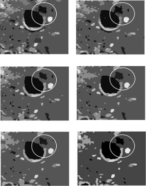
The second experiment was designed to evaluate the sensitivity of the segmentation result with differing initial conditions. We compared QHCF and uniform grid initialized HCF [19] (UGHCF) on human carotid MR images with a size of 128 pixels by 128 pixels. As UGHCF needs a predefined grid size, we chose 10, 20, and 30 pixels respectively. For the QHCF algorithm, the standard deviation of Quad-Tree region’s intensity was used as RC Vrc, and the threshold was adjusted at 5, 10, and 20 intensity levels, respectively. Other constraint parameters, such as β1 and β2 have same values for the two algorithms. Figure 8.5 is an example of the segmentation result processed with the above initial conditions. Although the overall performance of the two segmentation results seem quite similar given various input RC values, QHCF gives more consistent results than UGHCF (for example, the partitioned regions within the white dotted line circles are stable in QHCF under differing initialization).

8.2.4 Discussion and Conclusions

In this section, even though experimental results demonstrate that the QHCF leads to better segmentation results over other approaches, including UGHCF and adaptive ICM, same as what occurred in other random field based solutions, the determination of parameters including Trc, β1, β2, and Tmin is also a difficult part of implementing the QHCF into real applications. This is mainly because the evaluation of segmentation result is usually application oriented, which highly depends on the verifications of object identification/recognition at the higher level in the system. Therefore, it is hard to find an ideal measurement in the lower level to feedback the segmentation performance. Even though there is no theoretical approach on the automatic optimal searching, some heuristic solutions can be adopted in our implementation.

(i)Application-oriented empirical parameter selection: For different applications, the requirements of segmentation results may be different

Figure 8.5: Comparison of initialization sensitivity between UGHCF and QHCF. The original is in Fig. 7(a). (a)–(c) Segmentation results under uniform grid initialization with grid size 10, 20, and 30 pixels, respectively. (d)–(f) Results Reliability Criterion threshold Trc = 5, 10, and 20, respectively. The result within the white circle demonstrates the stability difference of the two algorithms with different initialization.

even with the same input image. Therefore, for a specific type of images, some empirical selections of parameters can be adopted. The parameters for two categories of images have been analyzed: one is about lumen segmentation with T1W MR images; the other is about the frame segmentation in videoconference clip. Table 8.1 shows the typical values of parameters in two applications for the QHCF algorithm.

Figure 8.6 is an example of the segmentation with different parameter combinations on T1W MR images. It shows that the parameter combination Trc = 10, Tmin = 10, β1 = 600, and β2 = 100 has better performance