

Kluwer - Handbook of Biomedical Image Analysis Vol
.2.pdf272 |
Yang and Mitra |
Control logic
V1 V2 |
Vc |
b11 b12 |
b21 |
bp2 bpc |
|
||
|
b22 |
|
|
b1c |
b2c bp1 |
Xj1 |
Xj2 |
Xjp |
Xj = {Xj1, |
Xj2, ..., Xjp} |
|
Recognition layer
Reset |
t |
|
Comparison layer
Figure 6.1: Adaptive fuzzy leader clustering (AFLC) structure.
The second layer serves as a verification process. By verifying the initial sample recognition through a vigilance test, the algorithm is able to dynamically create new clusters according to the data distribution when the verification fails, or optimize and update the system when the initial sample recognition is confirmed. The vigilance test consists of calculating a ratio between the distance of the sample to the winning cluster and the average distance of all the samples in this cluster to the cluster centroid,
R |
= |
|
|
x j − vi |
(6.2) |
|
Ni |
k=1 xk − vi |
|||
|
|
1 |
Ni |
|
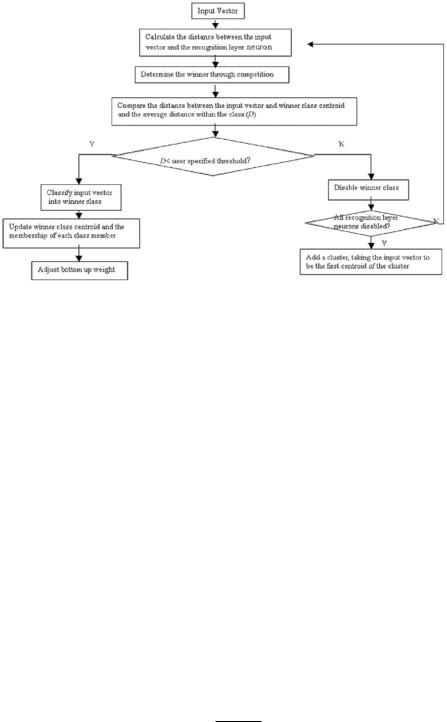
When this ratio is higher than a user-defined threshold, the test fails and a new cluster is created, taking the sample as the initial centroid and assigning an initial cluster distance value to this new cluster (which has only one sample coinciding with the centroid; it is necessary to assign an initial distance value so that the vigilance test can be performed when the next sample is presented). Otherwise, the sample is officially classified into this cluster, and then its centroid and the fuzzy membership values are updated with the following optimization parameters:
|
|
|
|
|
|
|
|
1 |
|
|
|
|
p |
|
||
|
|
|
|
|
|
|
|
|
|
|
|
|
|
|
||
|
vi = |
|
|
|
|
|
|
|
|
(uij )mx j i = 1, 2, . . . , c |
(6.3) |
|||||
|
|
|
p |
v |
|
(uij )m |
||||||||||
|
1/ x |
|
|
|
|
2 |
1/m−1 |
|
||||||||
uij = c |
1/ |
|
|
j=1 |
|
vk |
|
|
j=1 |
(6.4) |
||||||
|
x j |
|
|
|
2 |
|
1/m−1 i = 1, 2, . . . , c j = 1, 2, . . . , p |
|||||||||
|
|
|
|
j |
− |
|
i |
|
|
|
|
|
|
|||
|
k=1 |
|
|
|
|
|
− |
|
|
|
|
|
|
|||
Statistical and Adaptive Approaches for Optimal Segmentation |
273 |
Figure 6.2: Adaptive fuzzy leader clustering (AFLC) implementation flow chart.
The above nonlinear relationships between the ith centroid and the membership value of the jth sample to the ith cluster are obtained by minimizing the fuzzy objective function in Eq. (6.18). Figure 6.2 shows the flow chart for AFLC implementation. AFLC has been successfully applied to image restoration, image noise removal, image segmentation, and compression [13, 31, 32].
6.3.2 Deterministic Annealing
Deterministic annealing [13] is an optimization algorithm based on the principles of information theory, probability theory, and statistical mechanics. Shannon’s information theory tells us that the entropy of a system decreases as the underlying probability distribution concentrates and increases as the distribution becomes more uniform. For a physical system with many degrees of freedom that can result in many possible states. A basic rule in statistical mechanics says that when the system is in thermal equilibrium, possibility of a state i follows Gibbs distribution.
pi = |
e−Ei/ kB T |
(6.5) |
Z |
274 |
Yang and Mitra |
where kB is Boltzmann’s constant and Z is a constant independent of all states. Gibbs distribution tells us that states of low energy occur with higher probability than states of high energy, and that as the temperature of the system is lowered, the probability concentrates on a smaller subset of low energy states.
Let E be the average energy of the system, then
F = E − T H |
(6.6) |
is the “free energy” of the system. We can see that as T approaches zero, F approaches the average energy E. From the principle of minimal free energy, Gibbs distribution collapses on the global minima of E when this happens. SA [33] is an optimization algorithm based on Metropolis algorithm [34] that captures this idea. However, SA moves randomly on the energy surface and converges to a configuration of minimal energy very slowly, if the control parameter T is lowered no faster than logarithmically. DA improves the speed of convergence; the effective energy is deterministically optimized at successively reduced T while maintaining the annealing process aiming at global minimum.
In our clustering problem, we would like to minimize the expected distortion of all the samples x’s given a set of centroids y’s. Let D be the average distortion,
|
|
|
|
D = |
p(x, y)d(x, y) = |
p(x) p(y | x)d(x, y) |
(6.7) |
x y |
x |
y |
|
where p(x, y) is the joint probability distribution of sample x and centroid y, p(y | x) is the association probability that relates x to y, and d(x, y) is the distortion measure. Shannon’s entropy of the system is given by
H(X, Y) = − p(x, y) log p(x, y) (6.8)
If we take D as the average “energy” of the system, then the Lagrangian
F = D − T H, |
(6.9) |
is equivalent to the free energy of the system. The temperature T here is the Lagrange multiplier, or simply the pseudotemperature. Rose [13] described a probabilistic framework for clustering by randomization of the encoding rule, in which each sample is associated with a particular cluster with a certain probability. When F is minimized with respect to the association probability p(y | x),
Statistical and Adaptive Approaches for Optimal Segmentation |
275 |
|||||||
an encoding rule assigning x to y can be obtained, |
|
|
|
|||||
|
|
|
|
d(x, |
|
|
|
|
|
|
|
|
exp |
−d(x,y) |
|
|
|
p(y |
|
x) |
|
|
T |
|
|
(6.10) |
| |
= y exp |
− T |
|
|||||
|
|
|
|
|
y) |
|
|
|
Using the explicit expression for p(y | x) into the Lagrangian F in Eq. (6.9), we
have the new Lagrangian |
|
|
exp − d |
|
. |
|
|
x |
p(x) log |
y |
T |
(6.11) |
|||
|
|
|
|
|
(x, y) |
|
|
To get centroid values of {y}, we minimize F* with respect to y, yielding
d
p(x, y) |
|
d(x, y) = 0 |
(6.12) |
|
x |
dy |
|
With p(x, y) = p(x) p(y | x), where p(x) is given by the source and p(y | x) is also known (as given above.) The centroid values of y that minimize F* can be computed by an iteration that starts at a large value of T , tracking the minimum while decreasing T . The centroid rule is given by
yi = |
x |
xpp(yi) i | |
(6.13) |
|
|
|
(x) p(y |
x) |
|
where |
|
|
|
|
p(yi | x) = |
|
p(yi) e−(x−yi)2 / T |
|
||
k |
= |
|
(x yj )2 / T |
||
p |
i |
|
i | |
||
|
j |
=1 |
p(yj ) e− − |
||
|
|
|
|
|
|
(y ) |
|
p(x) p(y x) |
|||
x
(6.14)
(6.15)
It is obvious that the parameter T controls the entire iterative process of deriving final centroids. As the number of clusters increases, the distortion, or the covariance between samples x and centroids yi will be reduced. Thus, when T is lowered, existing clusters split and the number of clusters will increase while maintaining minimum distortion. When T reaches a value at which the clusters split, it corresponds to a phase transition in the physical system.
The exact value of T , at which a splitting will occur, is given by |
|
Tc = 2λmax |
(6.16) |
where Tc is known as the critical temperature and λmax is the maximum eigenvalue of the covariance matrix of the posterior distribution p(x | y) of the cluster
276 |
|
Yang and Mitra |
corresponding to centroid y: |
|
|
Cx | y = |
|
|
p(x | y)(x − y)(x − y)t |
(6.17) |
|
|
x |
|
In mass-constrained DA, the constraint of i pi = 1 is applied. Here pi’s are the centroids that coincide in the same cluster i at position yi. We call this the “repeated” centroids. This is because when the cluster splits, the annealing might result in multiple centroids in each effective cluster depending on the initial pertubation. Below is a simple description of implementation of DA:
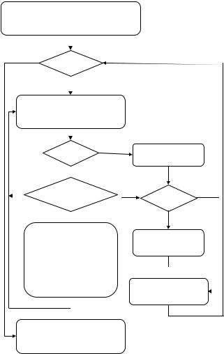
1.Initialization: set the maximum number of clusters to be generated Kmax and the minimum temperature Tmin. Set K = 1, compute the first Tc and first centroid. Set py1 = 1. Select temperature reduction rate α, perturbation δ, and threshold R.
2.For all current clusters, compute centroids yi and p(yi) according to Eqs. (6.13)–(6.15) until converge.
3.Check if T ≥ Tmin, if yes, reduce pseudotemperature T = αT , otherwise let T = 0 and stop, output centroids and sample assignments.
4.If K > Kmax, stop and output centroids and sample assignments. Otherwise, for all clusters, check if T > Tc(i), if yes, go to step 3; otherwise, split the cluster.
Figure 6.3 gives the flow chart for implementing mass-constrained DA. As can be seen from the flow chart, there are a couple of parameters that govern the annealing process, each exerts its influence on the outcome, particularly the temperature cooling step parameter α. Theoretically, if α is reduced sufficiently slowly, local minima of the cost function can be skipped and a global minimum can be reached. However, it can be very time consuming if T is reduced too slowly.
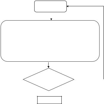
The centroids yi and the encoding rule p(yi | x) are illustrated in Fig. 6.4.
6.3.3 k-means Algorithm
k-means clustering [15] partitions a group of samples into K groups. The objective function to be reduced is the sum of square errors. The algorithm iterates as following:
Statistical and Adaptive Approaches for Optimal Segmentation |
277 |
Initialization
Kmax, T=Tc, K=1, py=1, a, d, R, r
N
K< Kmax
Y
T=a T, Update Tc(i),
i < K |
N |
K=K _current, i=1 |
|
 Y
Y
NT ≥ Tc(i)?
 Y
Y
Split cluster i:
K_current++, pyK_current=pyi/2,
pyi=pyi/2,
yK_current=yi+d,
i++
Stop,
output centroids yi & sample assignment
N
i < K
Y
Update
Eliminate
Notes
a: temperature cooling rate
d : perturbation
R: threshold value to eliminate repeated centroids
Update critical temperature: The critical temperature Tc for each cluster at temperature T is
calculated as in Tc =2λmax,
Figure 6.3: Flow chart for implementing mass-constrained deterministic an-
nealing (DA).
278 |
|
|
|
|
|
|
|
|
|
|
Yang and Mitra |
|
|
|
|
|
|
yi_old=yi |
|
|
|
|
|
|
|
∑x xp(x) p( yi | x) |
|
where |
p( yi ) = ∑ p(x) p( yi | x) |
||||||
|
= |
|
|
|
|
||||||
y i |
|
|
|
|
, |
|
|
x |
|
|
|
p( yi ) |
|
|
|
|
|
||||||
|
|
|
|
|
|
− (x − y i )2 |
|
|
|||
|
p ( yi | x) = |
|
|
p ( yi ) e |
/T |
||||||
|
|
|
|
|
|
||||||
|
|
|
K |
|
|
2 |
/T |
||||
|
|
|
|
|
|
|
|
||||
|
|
|
|
∑j = 1 p ( y j ) e |
− ( x − y j ) |
||||||
|
|
|
|
|
|
|
|||||
|
|
|
|| yi |
_ yi _ old || |
> R |
Y |
|||||
|
|| |
yi _ old || |
|
|
|
||||||
|
|
|
|
|
|
||||||
 N
N
Converge
Eliminate repeated centroids*f: discard centroids that coincide at the same location in one cluster:
For i =1:K,
If || yi − yj||/||yi||< R, then eliminate yj , py i = pyi +ypj , j =1:K
End
Figure 6.4: Mass-constrained deterministic annealing (DA) centroid update.
1.Compute the mean of each cluster as the centroid of that cluster.
2.Assign each sample to its closest cluster by calculating distances among the sample and all cluster centroids.
3.Keep iterate over the above two steps till the sum of square error of each cluster can no longer be reduced.
The initial centroids can be random; however, the choice of initial centroids is crucial and may result in incorrect partitioning. The iteration drives the objective function toward a minimum. The resultant grouping of the objects is geometrically as compact as possible around the centroids in each group.
Statistical and Adaptive Approaches for Optimal Segmentation |
279 |
6.3.4 Fuzzy C-Means
Fuzzy C-means [16] is a fuzzy version of k-means to include the possibility of having membership of the samples in more than one cluster. The goal is to find an optimal fuzzy c-partition that minimizes the objective function
n |
c |
|
|
|
|
Jm(U, V ; X) = |
(uij )m x j − vi 2 |
(6.18) |
j=1 i=1
where vi is the centroid of the ith cluster; uij is the membership value vector of the ith class for the jth sample; dij is the Euclidean distance between the ith class and sample x j ; c and n denote the number of classes to be clustered and the total number of samples, respectively; and m is a weighting exponential parameter on each fuzzy membership with1 ≤ m < ∞. The FCM algorithm can be described as follows:
1.Initialize membership function U(l=0) to random values.
2.Compute the centroid of the ith class with Eq. (6.3).
3.Update membership function U(l) with Eq. (6.4).
,,
4.If ,U(l−1) − U(l), ≤ ε or a predefined number of iteration is reached, stop. Otherwise l = l + 1 and go to step 2. ε is a small positive constant.
6.4 Results
We have chosen three different modalities of images, namely, MRI, stereo fundus images, and color cervix images to demonstrate the effectiveness of the advanced clustering algorithms over the traditional ones in segmenting medical images of various modalities.
6.4.1 MRI Segmentation
MRI is one of the most common diagnostic tools in neuroradiology. In brain pathology study, brain and brain tissues have often regions of interest from which abnormality such as the Alzheimer disease or multiple sclerosis (MS) lesions are diagnosed. Numerous techniques in computer-aided extraction of the brain, brain tissues, such as the gray matter, white matter, and cerebrospinal
280 |
Yang and Mitra |
fluid (CSF), as well as MS lesions have been developed [5, 8, 9, 35–38]. A good survey in applying pattern recognition techniques to MR image segmentation is available in [8]. Clark et al. [38] give a comparative study of fuzzy clustering approaches, including FCM and hard c-means versus supervised feedforward back-propagation computational neural network in MRI segmentation. These techniques are found to provide broadly similar results, with fuzzy algorithms showing better segmentation.
MS is a disease that affects the central nervous system. It affects more than 400,000 people in North America. Patients with MS experience range of symptoms depending on where the inflammation and demyelination is situated in the central nervous system. It can be from blurred vision, pain, affecting the sense of touch to loss of muscle strength in arms and legs. About 95% MS lesions occur in the white matter in the brain [39]. MR imaging is usually used to monitor the progression of the disease and the effect of drug therapy. Clinical analysis or grading of MS lesions is mostly performed by experienced raters visually or qualitatively. The involvement of such manual segmentation suffers from inconsistency between raters and inaccuracy. Computer aided automatic or semiautomatic segmentation of MS lesions in MR images is important in enhancing the accuracy of the measurement, facilitating quantitative analysis of the disease [35, 36, 39–43].
Many regular image segmentation techniques can be employed in MS lesion segmentation, such as edge detection, thresholding, region growing, and model-based approaches. However, because of MR field inhomogeneities and partial volume effect, most of the methods are integrated in nature, in which preand postprocessing are involved to correct these effects and remove noise, or a priori knowledge of the anatomical location of brain tissues is used [36, 39, 41]. Johnston et al. [35] used a stochastic-relaxation-based method, a modified iterated conditional modes (ICM) algorithm in 3D [6] on PDand T2-weighted MR images. Inhomogeneities in multispectral MR images are corrected by applying homomorphic filtering in the preprocessing step. After initial segmentation is obtained, a mask containing only the white matter and the lesion is generated by applying multiple steps of morphological filter and thresholding, on which a second pass of ICM is performed to produce the final segmentation. Zijdenbos et al. [36] applied back-propagation neural network for segmentation on both T1-, T2-, and PD-weighted images. Intensity inhomogeneities are corrected by using a so-called thin-plate spline surface fitted to the user-supplied reference points.
Statistical and Adaptive Approaches for Optimal Segmentation |
281 |
Noise is filtered before segmentation is performed by using an anisotropic diffusion smoothing algorithm [44]. An automatic method proposed by Leemput et al.
[45] removes the need for human interaction by using a probabilistic brain atlas for segmenting MS lesions from T1-, T2-, and PD-weighted images. This method simultaneously estimates the parameters of a stochastic tissue intensity model for normal brain MR images and detects MS lesions as voxels that are not fitted to the model.
6.4.1.1Normal Brain Segmentation from MRI: Gray Matter, White Matter, or Cerebrospinal Fluid
The intensity level and contrast can be very different for T1-, T2-, or PD-weighted MR images. Segmentation of gray matter, white matter, or CSF in the spatial domain depends highly on the contrast of the image intensity; therefore, T1weighted MRI is more suitable than T2or PD-weighted MRI. In order to validate the performances of the clustering algorithms, synthetic MRI [46, 47] is used because the existence of an objective truth model is helpful in obtaining quantative analysis of a segmentation technique, excluding the introduction of human error. The synthetic images used in this example are obtained from a simulated brain database [46, 47] provided by McConnell Brain Imaging Center, Montreal´ Neurological Institute, McGill University. It includes databases for normal brain and MS lesion brain. Three modalities are provided, T1-, T2-, and PD-weighted MRI. Simulations such as noise and intensity nonuniformity are also available.
The image in this example is #90 of 1-mm thick slices with 3% noise and 0% intensity nonuniformity. Figures 6.6–6.9 compare the segmentation results from DA, AFLC, FCM, and k-means. Misclassification, using the computer-generated truth model as the reference, is considered as the performance evaluation criterion following the traditional trend. Misclassification on each segmented category is calculated as the percentage of the total number of misclassified pixels in the segmented image divided by the total number of pixels in the corresponding truth model. For example, for the CSF, let class csf be the binary segmented image and csf model be the binary CSF truth model image,
N miss = total number of misclassification = sum (abs (class csf-csf model)) P model = total number of pixels in the CSF truth model = sum (csf model)
Misclassification = N miss/P model 100%