

Kluwer - Handbook of Biomedical Image Analysis Vol
.2.pdf202 |
Kallergi, Hersh, and Manohar |
8.Collect all imaging information and imaging parameters associated with selected cases.
9.Obtain all available reports, e.g., radiology, pathology, clinical reports, that can assist the researcher in case documentation and evaluation of the database contents.
For our development and preliminary study, data were collected retrospectively from the patient files of the H. Lee Moffitt Cancer Center & Research Institute. Approximately 100 patients undergo a pancreatic CT exam annually at the center. About 2/3 of these patients are diagnosed with pancreatic cancer and about 1/3 with a benign pancreatic mass or cyst. Abdominal scans are also performed for staging patients diagnosed with other cancer types, e.g., breast cancer, that may turn out to be negative for metastatic disease or any disease. Figure 4.9 shows a database design for pancreatic cancer imaging applications.
CT Images
(X+Y+Z)
Common percentages for Normal, Benign and Malignant cases
Sex |
|
|
Race |
|
Weight and Height |
|
Age |
|
|
Male |
(50%) |
|
Black and Hawaiian(50%) |
|
Fat |
(20%) |
|
< 50 |
(10%) |
Female |
(50%) |
|
White and Others (50%) |
|
Normal |
(60%) |
|
50 –70 |
(50%) |
|
|
|
|
|
Thin |
(20%) |
|
> 70 |
(40%) |
|
|
|
|
|
|
|
|
|
|
Normal |
|
|
|
Benign |
|
|
|
Malignant |
|
|
|
|||||
X |
|
|
|
Y |
|
|
|
|
Z |
|
|
|
|
|||
|
|
|
|
|
|
|
|
|
|
|
|
|
|
|
|
|
|
|
|
|
|
|
|
|
|
|
|
|
|
|
|
|
|
|
|
Mass |
|
|
|
|
Cysts |
|
|
|
|
|
|
|
|
|
|
|
|
|
|
|
|
|
|
|
Tumor size |
|
|||||
|
|
|
|
|
|
|
|
|
|
|
||||||
|
|
|
|
|
|
|
|
|
|
< 4 cm (50%) |
|
|||||
|
|
|
|
|
|
|
|
|
|
> 4 cm |
(50%) |
|
|
|||
|
|
|
|
|
|
|
|
|
|
|
|
|
|
|||
|
|
|
|
|
|
Head |
|
Body |
|
|
Tail |
|
Diffused |
|||
|
|
|
|
|
60% |
|
15% |
|
|
5% |
|
20% |
||||
|
|
|
|
|
|
|
|
|
|
|
|
|
|
|
|
|
Location of Tumor on the Pancreas
Figure 4.9: Image database design for pancreatic cancer research and CAD
development.
Automatic Segmentation of Pancreatic Tumors in Computed Tomography |
203 |
The contents of the database, e.g., numbers X, Y, and Z, are determined based on (a) the aims of the project, (b) the clinical characteristics of the pancreatic cancer and benign pancreatic masses, (c) the disease statistics, (d) the demographic characteristics both nationally and locally, (e) the imaging protocols implemented at the Institution, and (f) the requirements of the algorithm design as discussed earlier. Imaging protocols and surveillance procedures may differ among institutions and, hence, CAD goals may differ to accommodate specific clinical practices and requirements. HLMCC’s imaging protocol for abdominal helical CT scans of patients diagnosed with or suspected of pancreatic cancer includes three imaging series:
Series #1: An initial abdominal scan is done with a relatively thick slice (8–10 mm) prior to the administration of contrast material; approximately 5 slices from this series contain information of the pancreas.
Series #2: An enhanced abdominal scan follows with the same slice thickness as in Series #1 shortly after the intravenous administration of contrast material (a second enhanced scan after a short period of time may also be acquired if requested by the physician). Similar to the first series, approximately 5 slices in this series contain information on the pancreas.
Series #3: A high-resolution scan of the pancreas at a 4 mm or smaller slice thickness. This scan is not routinely performed and depends on the patient and the physician. This series consists of about 10 slices through the pancreas.
Series #4: A renal delay scan that acquires images through the kidneys only. This series includes partial information on the pancreas.
Series #1 and #4 are not likely to be of value at least in the initial algorithm development because pancreatic tumors are clinically evaluated in contrast enhanced scans, i.e., Series #2, and insufficient information is present in Series #4.
In addition to the CT images and imaging parameters, the following information was also collected or generated: (a) radiology reports, (b) pathology reports, (c) demographic information, (d) other nonimage information including lab tests, and (e) electronic ground truth files. All data were entered in a relational database that links image and nonimage information. All patient

204 |
Kallergi, Hersh, and Manohar |
identifiers were removed prior to any research and processing to meet confidentiality requirements.
4.4.2 Electronic Ground Truth File Generation
Ground truth files are and should be generated by physicians that are experts in the specific imaging modality and anatomy, e.g., CT interpretation and pancreatic disease. Despite subjectiveness and variability concerns, manual outlines by human experts are often the only way to establish ground truth or a form of ground truth to which image segmentation techniques can be compared to. If pathology information is available, as in the case of patients undergoing surgery or biopsy, then it can be used to provide stronger evidence on the true tumor size and possibly shape although the two sources of information, radiology and pathology, are not directly correlated. Unfortunately, in the case of pancreatic cancer, many of the tumors will not be resectable and will only undergo treatment; actually these are the patients one is most interested in, if one wants to determine treatment effects and tumor response over time. As a result, manual outlines by experts are the only option for ground truth generation on helical CT scans of the pancreas.
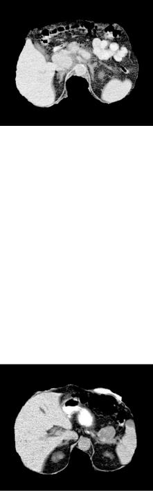
Figures 4.10(a) and 4.10(b) show two tumor outlines generated independently for the same CT slice and the same case with a malignant mass at the
Figure 4.10: (a) Two manual outlines of the pancreatic tumor shown in Fig. 4.6(a). (b) Two manual outlines of the pancreatic tumor shown in Fig. 4.7(a).
Automatic Segmentation of Pancreatic Tumors in Computed Tomography |
205 |
head and tail of the pancreas respectively (original images shown in Figs. 4.6(a) and 4.7(a)). These outlines are part of the ground truth files generated for the CT slices and used for segmentation validation. Variations in the outlines as the ones seen in Fig. 4.10 are expected and inevitable between experts and could make segmentation validation a strenuous task. Often there is no right or wrong answer and it is our recommendation that both are considered in an evaluation process.
Measures can and should be taken to increase the accuracy of this information and at a minimum remove external sources of variability or error. These measures include the following:
(i)Establish optimum and standard viewing and outline conditions in terms of monitor display and calibration, ambient light, manual segmentation tool(s), and image manipulation options.
(ii)Use all individual manual outlines for evaluation as a possible way to account for expert variability. For example, use both outlines shown in Fig. 4.10 for segmentation validation. Alternative options are to determine the union or overlap of outlines or use a panel of experts to obtain a consensus on one outline per image.
(iii)Provide all available information to the expert before he/she generates truth file.
(iv)Have experts perform initial outlines independently to avoid bias (any joint outlines are done in addition to the originals).
(v)Review the expertise of the “experts” and their physical condition prior to the initiation of the process (number of cases read within a certain time frame, familiarity with computer tools, training, fatigue).
(vi)Establish standard criteria and conventions to be followed by all experts in their outlines.
Ground truth files are generated for all cases in the designed database but for a selected number of image series and slices to reduce physician effort. Specifically, in the cases where there is no high-resolution series (#3), ground truth files are generated for the 5 enhanced CT slices of Series #2 that contain the pancreas. In the cases where the high-resolution series (#3) is available,
206 |
Kallergi, Hersh, and Manohar |
ground truth files are generated for both the 8 mm slices of the pancreas in Series #2 and every other slice in Series #3 (10 slices total); “ground truth” for the intermediate slices of Series #3 is obtained by interpolation. (Ground truth could be extrapolated from the 4 mm slices to the 8 mm slices but slice registration would be required prior to this process.)
Truth files are images of the same size as the original slice and include (a) the location of the pancreas and outline of its shape; (b) the location of the pancreatic tumor(s), masses, or cysts, and their shape outline(s) (Fig. 4.10);
(c) the location and identification of neighboring organs and their shape outlines; (d) the identification of any vascular invasion and metastases sites and outlines. Truth files are generated using a computer mouse to outline the areas of interest on CT slices that are displayed on a high resolution (2048 × 2560 pixels) and high luminance computer monitor. Pixels in the ground truth files are assigned a specific value that corresponds to an outlined organ or structure, e.g., a gray value of 255 is assigned to the pixels that correspond to the outline of the pancreatic tumor(s), a gray value of 200 to the pixels that correspond to the outline of the normal pancreas, etc.
4.4.3 External Signal Segmentation
The approach that was implemented was based on edge detection, line tracing, and histogram thresholding techniques [43]. The requirements for this process do not differ significantly from those followed in standard chest radiography (CXR) and several of the concepts described in CXR literature are applicable to CT as well [62]. One primary issue in this module was the desired level of accuracy in the removal of the external signals, i.e., signals from the rib cage and spine. Increasing the accuracy level, increased the computational requirements and the complexity of the methodology. Figures 4.11 and 4.12 show the external signal removal for the slices of Figs. 4.6(a) and 4.7(a).
A histogram equalization approach was used to remove the regions that correspond to the rib cage and spine that usually are the highest intensity regions in the image. Points on the rib cage were defined using the pixel characteristics of the rib cage and these points were interpolated using a spline interpolation technique [63]. The boundary of the rib cage was then estimated and removed.
Automatic Segmentation of Pancreatic Tumors in Computed Tomography |
207 |
Figure 4.11: External signal segmentation for the slice of Fig. 4.6(a).
4.4.4 Preprocessing—Enhancement
Our enhancement approach aimed at increasing the image contrast between the pancreas and organs in close proximity. A histogram equalization approach was implemented for this purpose and yielded satisfactory results (Gaussian and Wiener filters seemed to benefit these images as well) [64]. Wavelet-based enhancement was also considered as an alternative option for removing unwanted background information and better isolating the signals of interest [65]. The method was promising but may present an issue when used in combination with registration or reconstruction processes.
Enhancement generally benefits CAD algorithms but in 3-D imaging modalities like CT, it may have an adverse effect on the registration of the 2-D data, if it is not uniformly done across slices. Wavelet-based enhancement may worsen
Figure 4.12: External signal segmentation for the slice of Fig. 4.7(a).
208 |
Kallergi, Hersh, and Manohar |
the situation since it operates in the frequency domain and may not necessarily preserve the spatial features of the CT images as needed for registration. A standardization or normalization method may offer a solution in regaining all spatial information when transforming from the frequency back to the spatial domain. However, no such method was established for this application or is readily available. If registration is not part of the process, the enhancement step could significantly benefit subsequent clustering and classification on the CT images [66].
4.4.5 Fuzzy Clustering
A cluster or a class may be defined as a set of objects with similar characteristics (features) and different from other objects outside the group. When data are clustered, a condition is chosen for measuring the similarity of an object to that cluster. There are three types of clustering techniques: crisp, also known as hard or classical clustering, fuzzy, and probabilistic clustering [43, 48].
Crisp or classical clustering algorithms classify objects as part of a cluster or not part of a cluster. The object usually takes a hard value of either 0 or 1 with respect to a cluster or class. Cluster separation is very clear and no overlap is allowed. In real applications, however, and medical imaging in particular, there is overlap between the various data types and there are no crisp boundaries between classes.
Fuzzy clustering algorithms allow for data overlap because they use class membership values instead of binary assignments. These algorithms treats an object, e.g., an image pixel, as part of all clusters. The object is given a weight with respect to each cluster and the weight vector is unconstrained taking a value between 0 and 1. A weight greater than 0.5 indicates that the object is more likely to be similar to that cluster.
Probabilistic clustering is similar to fuzzy clustering with the exception of the weight vector being constrained in this case. Namely, the sum of all weights assigned to an object equals 1.
Various fuzzy clustering models are proposed in the literature. One widely used model is the fuzzy c-means (FCM) algorithm developed by Bezdek [48]. We have implemented FCM in several variations mainly for MRI brain tumor classification. Variations include unsupervised FCM [67, 68], FCM combined with knowledge based clustering [51], FCM combined with validity guided

Automatic Segmentation of Pancreatic Tumors in Computed Tomography |
209 |
(re)clustering [50], semisupervised FCM (ssFCM) algorithms [49], and supervised FCM algorithms [52, 53]. In supervised learning, FCM is trained under complete supervision, namely the algorithm is forced to learn every class correctly. In unsupervised learning, data are clustered according to their similarity, there is no forced training, and the algorithm is allowed to make its own classification decision. Semisupervised learning offers a middle path between the previous two. In this case, the user defines a degree of supervision that leaves some room for the algorithm to make its own decisions while not entirely unrestricted to do so. Semisupervised learning may offer advantages for the clustering of data with significant overlap. In the following paragraphs we will discuss few key theoretical aspects of the three learning approaches.
The FCM family of objective functions is defined as [47]
n |
c |
|
|
J(U, V ) = |
(uik)m xk − vi 2A |
k=1 i=1
where m [1, ∞) is a weighing exponent on each fuzzy membership, U Mfcn is a constrained fuzzy c-partition of the dataset X of n feature vectors xj in c clusters, V = (v1, v2, . . . , vc) are c-vector prototypes in the p-dimensional feature space Rp and A is any positive definite ( p × p) matrix. U and V may minimize
J only if
|
|
j |
c |
|
|
|
|
− |
|
2 |
|
−1 |
|
|
|
|
|
|
|
|
|
|
|
||||||||
uik |
= |
|
|
|
|
|
1 ≤ i ≤ c |
1 ≤ k ≤ n |
(4.1) |
||||||
|
1 |
|
|
xk |
v j A |
|
|||||||||
|
|
|
|
|
|
− |
|
m−1 |
|
|
|
|
|||
|
|
|
|
|
xk |
vi |
A |
|
|
|
|
|
|||
|
|
|
|
|
|
|
|
|
|
|
|
|
|||
|
= |
= |
|
|
|
|
|
|
≤ ≤ |
|
|
|
|||
|
|
k 1(uik)m |
|
|
|
|
|||||||||
|
|
|
n |
|
(uik)mxk |
|
|
|
|
|
|
|
|||
v |
|
|
k=1 |
|
|
|
|
1 |
|
i |
|
c |
|
(4.2) |
|
i |
|
|
n |
|
|
|
|
|
|
|
|
|
|
|
|
Note that U |
is |
= |
|
|
matrix |
of the uik values |
2 |
= (xk − |
|||||||
a (c × n) |
and xk − vi A |
||||||||||||||
vi)T A(xk − vi). The steps followed in the implementation of the FCM algorithm are as follows [47]:
1.Input unlabeled dataset X = {x1, x2, . . . , xn}
2.Choose parameters c (number of clusters), T, A, m ≥ 1, and ε > 0
3.Initialize U0 M f cn randomly
4.Compute the {vi,0} from (2) for 1 ≤ i ≤ c
5.For t = 1, 2, . . . , T do
210 |
Kallergi, Hersh, and Manohar |
(i)computer {uik,t } from (1) for 1 ≤ K ≤ n
(ii)computer error as Ut − Ut−1
(iii)if error ≤ ε stop; else compute {vi,t } from (2)
(iv)continue to the next t
In an unsupervised method, all n label vectors are unknown during initialization. Once a condition is satisfied and the parameter c is selected, the algorithm stops and each row in the matrix U corresponds to a cluster that may or may not have a label [47]. To avoid problems associated with nonlabeled clusters, a supervised FCM may be used. To change an unsupervised to a supervised method, expert human intervention is required and two things may be done:
1.The operator selects the number of clusters c during initialization.
2.The operator assigns labels to the classes at termination.
The problematic aspects of a supervised approach are the need for high-quality labeled data and the variability introduced by human intervention. An alternative to the supervised and unsupervised versions of FCM is the semisupervised method where a small set of the data is labeled but the majority of the data is unlabeled. In ssFCM, we let
X |
= |
x1 |
, x2 , . . . , xn1 , x1 , x2 , . . . , xn2 . . . . , x1 |
, x2 |
, . . . , xnc |
, |
x1 , x2 , . . . , xnu |
|
||||||||||
|
|
1 |
1 |
1 2 2 |
2 |
c |
c |
c |
|
|
u u |
|
u |
|
||||
|
|
( |
|
|
|
)* |
|
|
|
|
+, ( |
|
)* |
|
+ |
|||
|
|
|
|
labeled data |
|
|
|
|
, |
|
|
|
|
|
||||
|
|
|
|
|
|
|
,unlabeled data |
|||||||||||
|
|
|
|
|
|
|
|
|
|
|
, |
|
|
|
|
|
|
|
denote partially labeled data; superscripts denote the class label and ni is the number of samples having the same label vector in the partition matrix U . Using the labeled set of data we find the center of the clusters iteratively until the terminating condition is satisfied. The unlabeled data are then introduced for finding the cluster centers. This method is more stable as the centers are well defined from the labeled data used for training. The clusters are also well defined with the correct physical data labels.
The cluster centers for the labeled data are calculated as
|
= |
|
kd |
|
1 |
(uikd |
,0)m |
|
≤ ≤ |
|
||
|
|
|
nd |
|
|
d |
|
) |
m d |
|
|
|
|
|
|
k=1 |
(u |
|
x |
|
|
|
|||
vi,0 |
|
|
n |
|
|
|
|
|
|
1 |
i c |
(4.3) |
|
|
= |
|
|
|
|
|
|
|
|
||
where the subscript d denotes design or training data. Having the labels for the
Automatic Segmentation of Pancreatic Tumors in Computed Tomography |
211 |
nd points, we need to update only the nu columns in U by calculating:
|
|
|
|
|
|
|
u |
|
|
|
|
|
|
2 |
|
−1 |
|
|
ik,t |
= |
j=1 |
|
|
|
|
|
|
|
m−1 |
≤ ≤ ≤ ≤ |
= |
||||||
|
|
|
|
|
|
|
|
|
||||||||||
|
xku |
− |
v j,t |
1 |
|
A |
|
|||||||||||
uu |
|
|
c |
|
|
− |
|
|
1 i c 1 k nu t 1, 2, . . . , T |
|||||||||
|
|
|
|
xk |
− vi,t−1 |
A |
|
|
||||||||||
(4.4) Once the initial cluster centers {vi,0} are calculated, cluster centers are recomputed using the unlabeled data as
|
= |
|
|
|
k 1(uik,t )m |
|
|
k 1(uik,t )m |
|
|
≤ ≤ = |
||||
|
|
|
|
nd |
|
d |
m d |
+ |
|
nu |
u |
m |
u |
|
|
vi,t |
|
|
|
k=1(uik,t ) |
xk |
|
k=1 |
(uik,t ) |
xk |
1 |
i c t 1, 2, . . . , T (4.5) |
||||
|
|
|
nd d |
|
+ |
nu |
u |
|
|
||||||
|
|
|
= |
|
|
= |
|
|
|
|
|
||||
where the subscript u is now used to denote the unlabeled data contribution. In practice, nd is much smaller than nu. For example, an abdominal CT im-
age is usually 512 × 512 or 262,144 pixels. A pancreatic mass of about 4 cm in maximum diameter may cover approximately 1200 pixels in an image with a resolution of 1 mm/pixel while the pancreas itself may be up to 5000 pixels. Neighboring major organs and structures may be up to 20,000 pixels depending on the slice. A very small percentage of these pixels will be labeled in the ssFCM approach. For example for c = 4 a quarter of the pixels in each class per slice are labeled, which approximately equals to nd = 8000 and nu = 254,144.
To reduce potential bias that may be introduced by large differences between nd and nu as well as between the difference tissue classes, one more modification of c-means is introduced that allows us to weigh the fewer labeled samples more heavily than their unlabeled counterparts. Furthermore, such weighing allows us to assign much larger weights to small clusters to better separate them from larger ones. This is done by introducing weights W = (w1, w2, . . . , wnd) in the Eq. (4.5) as
|
|
|
|
nd |
|
d |
m d |
+ |
|
nu |
u |
m |
u |
|
|
|
|
|
|
|
|
Vi,t |
|
|
|
k=1 wk(uik,t ) |
xk |
|
k=1 |
(uik,t ) |
|
xk |
|
1 |
|
i |
|
c t |
|
1, 2, . . . , T |
|||
= |
|
|
|
nd |
d |
|
|
|
nu |
u |
|
|
≤ |
≤ |
= |
||||||
|
|
k 1 wk |
(uik,t )m |
|
k 1 |
(uik,t )m |
|
|
|
|
|||||||||||
|
|
|
= |
|
|
+ = |
|
|
|
|
|
|
|
|
|
|
|
||||
(4.6) In general, W is a vector of positive real numbers and when wnd = 1 then ssFCM becomes standard unsupervised FCM [47].
The implementation of an ssFCM algorithm involves the following steps:
1.Given partially labeled data X = Xd Xu, set the nd and nu parameters as nd = |Xd| and nu = |Xu|; the c parameter is known and fixed by the training data.