Kluwer - Handbook of Biomedical Image Analysis Vol

imposed on the computation of the normalized cross correlation:

Time-intensity curves similar to the reference curve will have high-correlation values and are bright in the similarity map, whereas those with low-correlation values are dark. Therefore, structures in the dynamic image sequence can be segmented from the similarity map based on their temporal changes rather than spatial similarities. It should be noted that cross-correlation does not depend on the absolute magnitude of the time-intensity curves. Regions whose timeintensity curves are differed from the reference curve r by an additive or by a multiplicative constant, will have a perfect positive correlation (+1).

By using different reference ROIs, a series of similarity maps containing different segmentation for regions that have similar or different temporal kinetics can be obtained. It was used to investigate local changes and segmentation of rabbit kidney on spatially aligned image sequences obtained from dynamic MR imaging of Gd-DTPA [64]. The similarity mapping technique has also been applied to brain activation studies to extract the activated regions and their temporal dynamics [65]. The same technique has also been used to segment the area of ischemia in the left coronary artery territory, lung tumor, and tentorial meningioma, and localize the focal ischemic region in brain [66].

3.5.3.2 Principal Component Analysis

Principal component analysis (PCA), also called Karhunen–Loeve´ transform or Hotelling transform, is probably the most famous method in multivariate data analysis [67]. It was developed independently by Pearson [68] in 1901 and Hotelling [69] in 1933. It has been widely applied in a number of scientific areas such as biology, chemistry, medicine, psychology, and the behavioral sciences. Given a set of multivariate data, PCA explains the variance–covariance structure by linearly transforming the (possibly) correlated variables into a smaller set of uncorrelated (orthogonal) variables called principal components (PCs). The first (highest order) component maximally accounts for the variation in the original data and each succeeding component maximally accounts for the remaining variation present in the original data. In other words, higher order components are important as they explain the major variation (also the feature) in

the data, whereas lower order components are unimportant as they mainly contain noise, which can be discarded without causing too much loss of information of the original data. Therefore, dimensionality reduction (or data compression) can be achieved using PCA technique. Separation of tissue types characterized by different features can also be accomplished by careful inspection of the PCs. This is because each PC contains only the representative feature that is specific to that PC and cannot be found elsewhere (theoretically) owing to orthogonality among PCs.

Let the dynamic sequence of images be represented by a matrix X that has M rows and N columns. Each column represents a time frame of image data and each row represents a pixel vector, i.e., a tissue TAC or a dixel [63], which is a time series xi as in Eqs. (3.15) and (3.17). Note that there is no explicit assumption on the probability density of the measurements xi as long as the first-order and second-order statistics are known or can be estimated from the available measurements. Each of xi can be considered as a random process

If the measurements (or random variables) xj are correlated, their major variations can be accurately approximated with less than N parameters using the PCA. The mean of x is given by

and the covariance matrix of the same dataset is given by

which is a N × N symmetric matrix. The elements of Cx, denoted by ckl , represent the covariances between the random variables xk and xl , whereas the element ckk is the variance of the random variable xk. If xk and xl are uncorrelated, their covariance would be zero, i.e., ckl = clk = 0. The mean and the covariance matrix of a sample of random vectors xi can be estimated from its sample mean and sample covariance matrix in a similar manner.

The orthogonal basis of the covariance matrix Cx can be calculated by finding its eigenvalues and eigenvectors. It is well known from basic linear algebra that the eigenvectors ek and the corresponding eigenvalues λk are the solutions of

for k = 1, 2, . . . , N and λk = 0. There are several numerical methods to solve for λk and ek in Eq. (3.26). One of the popular approaches is to make use of the symmetrical property of Cx and solve for the eigenvalues and eigenvectors by means of Householder reduction followed by QL algorithm with implicit shifts [70, 71]. As Cx is a real, symmetric matrix, an equivalent approach is to compute the singular value decomposition (SVD) of the matrix Cx directly:

where U is a N × N column-orthogonal matrix, V is a N × N orthogonal matrix that contains the eigenvectors, and Λ is a N × N diagonal matrix whose squared diagonal elements correspond to the eigenvalues. However, the difference between SVD and the eigen-decomposition should be noted, in particular, the eigen-decomposition of a real matrix might be complex, whereas the SVD of a real matrix is always real.

The ordering of the eigenvectors can be sorted in the order of descending eigenvalues such that λ1 ≥ λ2 ≥ · · · ≥ λN ≥ 0. In this way, an ordered orthogonal basis is formed, and the first eigenvector e1 (the one associated with λ1) has the direction of the largest variance of the data (the first PC), and the second eigenvector e2 has the direction of the second largest variance of the data (the second PC), and so on. The PCs are obtained by projecting the multivariate random vectors onto the space spanned by the eigenvectors. Let Ω be a matrix that stores the eigenvectors ek as row vectors, then the PCs, y = [y1, y2, . . . , yN ]T , can be calculated as

which defines a linear transformation for the random vector x through the orthogonal basis and x is calculated from Eq. (3.24). The kth PC of x is given by

which has zero mean. The PCs are also orthogonal (uncorrelated) to one another because

which indicates that the variances of the PCs are given by the eigenvalues of

Cx. As the PCs have zero means, a very small eigenvalue (variance) λk implies that the value of the corresponding PC is also very small to contribute to the total variances present in the data. Since the eigenvalue sequence {λk} is monotonically decreasing and typically the sequence drops rapidly, it is possible to determine a limit below which the eigenvalues (and PCs) can be discarded without causing significant error in reconstruction of the original dataset using only the retained PCs. Thus, data compression (or dimensionality reduction) can be achieved and this is an important application of PCA. Instead of using all eigenvectors of the covariance matrix Cx, the random vector x can be approximated by the highest few basis vectors of the orthogonal basis. Suppose that only the first K rows (eigenvectors) of Ω are selected to form a K × N matrix, ΩK , a similar transformation as in Eqs. (3.28) and (3.31) can be derived

where y˜ represents a truncated PC vector, which contains only the K highest PCs, and xˆ is an approximation of x with the K highest PCs. It can be shown that the mean square error (MSE) between xˆ and x is given by

N

The practical issue here is the choice of K beyond which the PCs are insignificant. The gist of the problem lies in how “insignificant” is defined and how much error one could tolerate in using less number of PCs to approximate the original data. Sometimes, a small number of PCs are sufficient to give an accurate approximation to the observed data. A commonly used strategy is to plot the eigenvalues against the number of PCs and detect a cut-off beyond which the eigenvalues become constants. Another approach is to discard the PCs with eigenvalues lower than a specified fraction of the first (largest) eigenvalue. There is no simple answer and one has to trade off between errors and the number of PCs for approximation of the observed data which is the primary concern when PCA is used for data compression.

PCA has been applied to analyze functional images including nuclear medicine [72–77] and dynamic MRI [78, 79] where data visualization, structure and functional classification, localization of diseases, and detection of activation patterns are of primary interests. Moeller and Strother [72] applied PCA to analyze functional activation patterns in brain activation experiments. Strother et al. [75] revealed an intraand intersubject subspace in data and demonstrated that the activation pattern is usually contained in the first PC. A later study conducted by Ardekani et al. [76] further demonstrated that the activation pattern may spread across several PCs rather than lie only on the first PC, particularly when the number of subjects increases and/or multicenter data are used. PCA was also applied to aid interpretation of oncologic PET images. Pedersen et al. [74] applied PCA to aid analyze of dynamic FDG-PET liver data. Anzai et al. [77] investigated the use of PCA in detection of tumors in head and neck, also using dynamic FDG-PET imaging. It was found that the first few highest order component images often contained tumors whereas the last several components were simply noise.

Absolute quantification of dynamic PET or SPECT data requires an invasive procedure where a series of blood samples are taken to form an input function for kinetic modeling (Chapter 2 of Handbook of Biomedical Image Analysis: Segmentation, Volume I). Sampling blood at the radial artery or from an arterialized vein in a hand is the currently recognized method to obtain the input function. However, arterial blood sampling is invasive and has several potential risks associated with both the patient and the personnel who performed the blood sampling [80]. Drawing ROI around vascular structures (e.g., left ventricle in the myocardium [81] and internal carotid artery in the brain [82]) has been

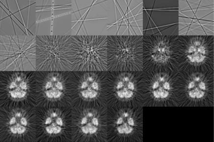
Figure 3.2: A sequence of dynamic neurologic FDG-PET images sampled at the level where the internal carotid arteries are covered. Individual images are scaled to their own maximum.

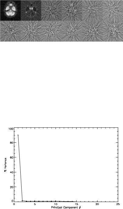
proposed as a noninvasive method that obviates the need of frequent blood sampling. Delineation of larger vascular structures in the myocardium is relatively straightforward. In contrast, delineation of internal carotid artery in the head and neck is not trivial. A potential application of PCA is the extraction of input function from the dynamic images in which vascular structures are present in the dynamic images. Figure 3.2 show a sequence of dynamic neurologic FDGPET images sampled at the level in the head where the internal carotid arteries are covered. Figure 3.3 shows the highest 12 PC images. The signal-to-noise ratio (SNR) of the first PC image is very high when comparing with the original image sequence. For PC images beyond the second, they simply represent the remaining variability that the first two PC images cannot account for and they are dominated by noise. The internal carotid arteries can be seen in the second PC image which can be extracted by means of thresholding as mentioned before in sections 3.4.1 and 3.4.4. Figure 3.4 shows a plot of percent contribution to the total variance for individual PCs. As can be seen from the figure, the first and the second PCs contribute about 90% and 2% of the total variance, while the remaining PCs only contribute for less than 0.6% of the total variance individually.

Figure 3.3: From left to right, the figure shows the first six principal component (PC) images (top row), and the 7th to 12th PC images (bottom row) scaled to their own maxima. All but the first two PC images are dominated by noise. The higher order PC images (not shown) look very similar to PC images 3–12.

This means that large amount of information (about 92%) is preserved in only the first two PCs, and the original images can be approximated by making use only the first one or two PCs.

Different from model-led approaches such as compartmental analysis where the physiological parameters in a hypothesized mathematical model are estimated by fitting the model to the data under certain possibly invalid assumptions, PCA is data-driven, implying that it does not rely on a mathematical model.

Figure 3.4: The percent variance distribution of the principal component (PC)

images.

Instead, it explores the variance–covariance structure of the observed data and finds a set of optimal (uncorrelated) PCs, each of which contains maximal variation present in the measured data. A linear combination of these components can accurately represent the observed data. However, because of lack of model as a constraint, PCA cannot separate signals from statistical noise, which may be an important component if it is highly correlated and dominates the multivariate data. In this case, convincing results of dimensionality reduction or structure exploration may not be achievable as noise is still retained in the higher order components. In addition, the orthogonal components produced by PCA are not necessarily physiological meaningful. Thus, it is difficult to relate the extracted components to the underlying TACs and structures in the multivariate data.

3.5.3.3 Factor Analysis

Factor analysis of dynamic structures (FADS), or factor analysis (FA), can be thought of as a generalization of PCA as it produces factors closer to the true underlying tissue response and assumes a statistical model for the observed data. FADS is a semiautomatic technique used for extraction of TACs from a sequence of dynamic images. FADS segments the dynamic sequence of images into a number of structures which can be represented by functions. Each function represents one of the possible underlying physiological kinetics such as blood, tissue, and background in the sequence of dynamic images. Therefore, the whole sequence of images can be represented by a weighted sum of these functions.

Consider a sequence of dynamic images X of size M × N, with M being the number of pixels in one image and N the number of frames. Each row of X represents a pixel vector, which is a tissue TAC in PET/SPECT data. Assume that pixel vectors in X can be represented by a linear combination of factors F, then X can written as

where C contains factor coefficients for each pixel and it is of size M × K with

K being the number of factors; F is a K × N matrix which contains underlying tissue TACs. The additive term η in Eq. (3.36) represents measurement noise in X.

Similar to the mathematical analysis detailed before for similarity mapping and PCA, we define xi as the ith pixel vector in X, and fk being the kth underlying

factor curve (TAC), and cki being the factor coefficient that represents contribution of the kth factor curve to xi. Let Y = CF and yi be a vector which represents the ith row of Y, then

K

and

where ηi represents a vector of noise associated with xi. Simply speaking, these equations mean that the series of dynamic images X can be approximated and constructed from some tissue TACs of the underlying structures (represented by a factor model Y = CF), which are myocardial blood pools, myocardium, liver, and background for cardiac PET/SPECT imaging, for example. The aim of FADS is to project the underlying physiological TACs, yi as close as possible to the measured TACs, xi, so that the MSE between them can be minimized:

Typically, FADS proceeds by first identifying an orthogonal basis for the sequence of dynamic images followed by an oblique rotation. Identification of the orthogonal basis can be accomplished by PCA discussed previously. However, the components identified by PCA are not physiologically meaningful because some components must contain negative values in order to satisfy the orthogonality condition. The purpose of oblique rotation is to impose nonnegativity constraints on the extracted factors (TACs) and the extracted images of factor coefficients [63].

As mentioned in section 3.2, careful ROI selection and delineation are very important for absolute quantification, but manually delineation of ROI is not easy due to high-noise levels present in the dynamic images. Owing to scatter and patient volume effects, the selected ROI may represent “lumped” activities from different adjacent overlapping tissue structures rather than the “pure” temporal behavior of the selected ROI. On the other hand, FADS can separate partially overlapping regions that have different kinetics, and thereby, extraction of TACs corresponding to those overlapping regions is possible.

Although the oblique rotation yield reasonable nonnegative factor curves that are highly correlated with the actual measurements, they are not unique [83] because both factors and factor coefficients are determined simultaneously. It is very easy to see this point by a simple example. Assume that a tissue TAC x composes of only two factors f1 and f2 and c1 and c2 being the corresponding factor coefficients. According to Eqs. (3.36) and (3.37), x can be represented by

with some constant α. It can be seen that Eqs. (3.40) and (3.41) are equivalent for describing the measured TAC, x, as long as f1 + αf2 and c2 − αc1 are nonnegative if nonnegativity constraints have to be satisfied. In other words, there is no difference to represent x using factors f1 and f2 and factor coefficients c1 and c1, or using factors f1 + αf2 and f2 and factor coefficients c1 and c2 − αc1. Therefore, further constraints such as a priori information of the data being analyzed are required [84–87].

FADS has been successfully applied to extract the time course of blood activity in left ventricle from PET images by incorporating additional information about the input function to be extracted [88, 89]. Several attempts have also been made to overcome the problem of nonuniqueness [90, 91]. It was shown that these improved methods produced promising results in a patient planar

99mTc-MAG3 renal study and dynamic SPECT imaging of 99mTc-teboroxime in canine models using computer simulations and measurements in experimental studies [90, 91].

3.5.3.4 Cluster Analysis

Cluster analysis has been described briefly in section 3.4.4. One of the major aims of cluster analysis is to partition a large number of objects according to certain criteria into a smaller number of clusters that are mutually exclusive and exhaustive such that the objects within a cluster are similar to each others, while objects in different clusters are dissimilar. Cluster analysis is of potential value in classifying PET data, because the cluster centroids (or centers) are derived