Kluwer - Handbook of Biomedical Image Analysis Vol

down-weights observations that are atypical for the normal distribution, making the parameter estimation more robust against such outliers.

1.4.2 From Typicality Weights to Outlier Belief Values

Since each voxel j has only a contribution of t(yj | ) to the parameter estimation, the remaining fraction

reflects the belief that it is a model outlier. The ultimate goal in our application is to identify these outliers as they are likely to indicate pathological tissues. However, the dependence of Eq. (1.14) through t(yj | ) on the determinant of the covariance matrix Σ prevents its direct interpretation as a true outlier belief value.

In statistics, an observation y is said to be abnormal with respect to a given normal distribution if its so-called Mahalanobis distance

d = (y − µ)t Σ−1(y − µ)

exceeds a predefined threshold. Regarding Eq. (1.12), the Mahalanobis distance at which the belief that a voxel is an outlier exceeds the belief that it is a regular sample decreases with increasing |Σ|. Therefore, the Mahalanobis distance threshold above which voxels are considered abnormal changes over the iterations as Σ is updated. Because of this problem, it is not clear how λ should be chosen.

Therefore, Eq. (1.12) is modified into

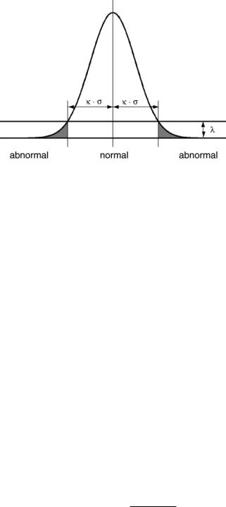
where |Σ| is explicitly taken into account and where λ is reparameterized using the more easily interpretable κ. This κ ≥ 0 is an explicit Mahalanobis distance threshold that specifies a statistical significance level, as illustrated in Fig. 1.15. The lower κ is chosen, the easier voxels are considered as outliers. On the other hand, choosing κ = ∞ results in t(yj | (m−1)) = 1, j which causes no outliers to be detected at all.

Figure 1.15: The threshold κ defines the Mahalanobis distance at which the belief that a voxel is a model outlier exceeds the belief that it is a regular sample (this figure depicts the unispectral case, where Σ = σ 2).

1.4.3 Robust Estimation of MR Model Parameters

Based on the same concepts, the EM framework used in the previous sections for estimating the parameters of models for normal brain MR images can be extended to detect model outliers such as MS lesions. In the original EM algorithm, a statistical classification f (l j | Y, (m−1)) is performed in the expectation step, and the subsequent maximization step involves updating the model parameters according to this classification. The weights f (l j = k | Y, (m−1)), k =

1, 2, . . . , K represent the degree to which voxel j belongs to each of the K tis-

for all tissue types simultaneously.

A similar approach as the one described above, where Eq. (1.9) was replaced with the more robust Eq. (1.11) and solved with a W-estimator, results in a maximization step in which model outliers are down-weighted. The resulting equations for updating the model parameters are identical to the original ones, provided that the weights f (l j | Y, (m−1)) are replaced everywhere with a combination of two weights f (l j | Y, (m−1)) · t(yj | l j , (m−1)), where

liers can have a small degree of membership in all tissue classes simultaneously. Therefore, observations that are atypical for each of the K tissue types have a reduced weight on the parameter estimation, which robustizes the EM-procedure. Upon convergence of the algorithm, the belief that voxel j is a model outlier is given by

1 − f (l j = k | Y, ) · t(yj | l j = k, ) (1.16)

k

Section 1.5 discusses the use of this outlier detection scheme for fully automated segmentation of MS lesions from brain MR images.

1.5 Application to Multiple Sclerosis

In [52], the outlier detection scheme of section 1.4 was applied for fully automatic segmentation of MS lesions from brain MR scans that consist of T1-, T2-, and PDweighted images. Unfortunately, outlier voxels also occur outside MS lesions. This is typically true for partial volume voxels that, in contravention to the assumptions made, do not belong to one single tissue type but are rather a mixture of more than one tissue. Since they are perfectly normal brain tissue, they are prevented from being detected as MS lesion by introducing constraints on intensity and context on the weights t(yj | l j , ) calculated in Eq. (1.15).

1.5.1 Intensity and Contextual Constraints

Since MS lesions appear hyperintense on both the PDand the T2-weighted images, only voxels that are brighter than the mean intensity of gray matter in these channels are allowed to be outliers.

Since around 90–95% of the MS lesions are white matter lesions, the contextual constraint is added that MS lesions should be located in the vicinity of white matter. In each iteraction, the normal white matter is fused with the lesions to form a mask of the total white matter. Using a MRF as in section 1.3, a voxel is discouraged from being classified as MS lesion in the absence of neighboring white matter. Since the MRF parameters are estimated from the data in each iteration as in section 1.3, these contextual constraints automatically adapt to the voxel size of the data.

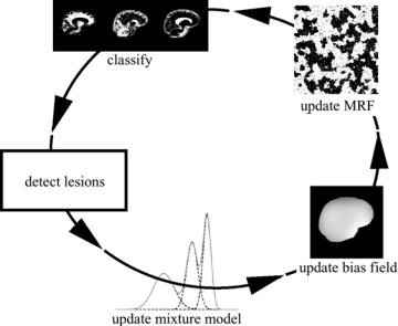
Figure 1.16: The complete method for MS lesion segmentation iteratively interleaves classification of the voxels into normal tissue types, MS lesion detection, estimation of the normal distributions, bias field correction, and MRF parameter estimation.

The complete method is summarized in Fig. 1.16. It iteratively interleaves statistical classification of the voxels into normal tissue types, assessment of the belief for each voxel that it is not part of an MS lesion based on its intensity and on the classification of its neighboring voxels, and, only based on what is considered as normal tissue, estimation of the MRF, intensity distributions, and bias field parameters. Upon convergence, the belief that voxel j is part of an MS lesion is obtained by Eq. (1.16). The method is fully automated, with only one single parameter that needs to be experimentally tuned: the Mahalanobis threshold κ in Eq. (1.15). A 3-D rendering of the segmentation maps including the segmentation fo MS lesions is shown in Fig. (1.17).

1.5.2 Validation

As part of the BIOMORPH project [57], we analyzed MR data acquired during a clinical trial in which 50 MS patients were repeatedly scanned with an interval of approximately 1 month over a period of about 1 year. The serial image data consisted at each time point of a PD/T2-weighted image pair and

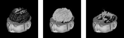
Figure 1.17: A 3-D rendering of (a) gray matter, (b) white matter, and (c) MS lesion segmentation maps. (Color slide)

a T1-weighted image with 5 mm slice thickness. From 10 of the patients, two consecutive time points were manually analyzed by a human expert who traced MS lesions based only on the T2-weighted images. The automatic algorithm was repeatedly applied with values of the Mahalanobis distance κ varying from 2.7 (corresponding to a significance level of p = 0.063) to 3.65 (corresponding to p = 0.004), in steps of 1.05. The automatic delineations were compared with the expert segmentations by comparing the so-called total lesion load (TLL), measured as the number of voxels that were classified as MS lesion, on these 20 scans. The TLL value calculated by the automated method decreased when κ was increased, since the higher the κ, the less easily voxels are rejected from the model. Varying κ from 2.7 to 3.65 resulted in an automatic TLL of respectively 150% to only 25% of the expert TLL. However, despite the strong influence of κ on the absolute value of the TLL, the linear correlation between the automated TLLs of the 20 scans and the expert TLLs was remarkable insensitive to the choice of κ. Over this wide range, the correlation coefficient varied between 0.96 and 0.98.

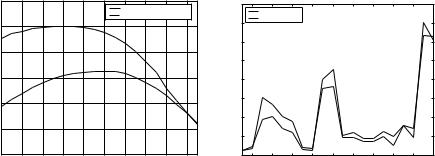
Comparing the TLL of two raters does not take into account any spatial correspondence of the segmented lesions. We therefore calculated the similarity index defined in Eq. (1.8), which is simply the volume of intersection of the two segmentations divided by the mean of the two segmentation volumes. For the 20 scans, Fig. 1.18(a) depicts the value of this index for varying κ, both with and without the bias correction step included in the algorithm, clearly demonstrating the need for bias field correction. The best correspondence, with a similarity index of 0.45, was found for κ 3. For this value of κ, the automatic TLL was virtually equal to the expert TLL, and therefore, a similarity index of

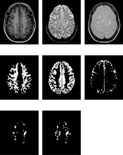
Figure 1.19: Automatic classification of one of the 20 serial datasets that were also analyzed by a human expert. (a) T1-weighted image; (b) T2-weighted image;

(c) PD-weighted image; (d) white matter classification; (e) gray matter classification; (f) CSF classification; (g) MS lesion classification; (h) expert delineation of the MS lesions. (Source: Ref. [52].)

pure tissue types for training an automated classifier [58–61]. While these methods have proven to be useful, they remain impractical when hundreds of scans need to be analyzed as part of a clinical trial, and the variability of manual tracings is not totally removed. In contrast, the method presented here is fully automated as it uses a probabilistic brain atlas to train its classifier. Furthermore the atlas provides spatial information that avoids nonbrain voxels from being classified as MS lesion, making the method work without the often-used tracing of the intracranial cavity in a preprocessing step [58–63].

A unique feature of our algorithm is that it automatically adapts its intensity models and contextual constraints when analyzing images that were acquired with a different MR pulse sequence or voxel size. Zijdenbos et al. described [64] and validated [65] a fully automated pipeline for MS lesion segmentation based on an artificial neural network classifier. Similarly, Kikinis, Guttmann et al.

[62, 66] have developed a method with minimal user intervention that is built on the EM classifier of Wells et al. [4] with dedicated preand postprocessing steps. Both methods use a fixed classifier that is trained only once and that is subsequently used to analyze hundreds of scans. In clinical trials, however, interscan variations in cluster shape and location in intensity space cannot be excluded, not only because of hardware fluctuations of MR scanners over a period of time, but also because different imagers may be used in a multicenter trial [66]. In contrast to the methods described above, our algorithm retrains its classifier on each individual scan, making it adaptive to such contrast variations.

Often, a postprocessing step is applied to automatically segmented MS lesions, in which false positives are removed based on a set of experimentally tuned morphologic operators, connectivity rules, size thresholds, etc. [59, 60, 62]. Since such rules largely depend on the voxel size, they may need to be retuned for images with a different voxel size. Alternatively, images can be resampled to a specific image grid before processing, but this introduces partial voluming that can reduce the detection of lesions considerably, especially for small lesion loads [66]. To avoid these problems, we have added explicit contextual constraints on the iterative MS lesions detection that automatically adapt to the voxel size. Similar to other methods [59, 61, 63, 64], we exploit the knowledge that the majority of MS lesions occurs inside white matter. Our method fuses the normal white matter with the lesions in each iteration, producing, in combination with MRF constraints, a prior probability mask for white matter that is automatically updated during the iterations. Since the MRF parameters are

reestimated for each individual scan, the contextual constraints automatically adapt to the voxel size of the images.

Although the algorithm we present is fully automatic, an appropriate Mahalanobis distance threshold κ has to be chosen in advance. When evaluating the role of κ, a distinction has to be made between the possible application areas of the method. In clinical trials, the main requirement for an automated method is that its measurements change in response to a treatment in a manner proportionate to manual measurements, rather than having an exact equivalence in the measurements [67, 68]. In section 1.5.2 it was shown that the automatic measurements always kept changing proportionately to the manual measurements for a wide range of κ, with high correlation coefficients between 0.96 and 0.98. Therefore, the actual choice of κ is fairly unimportant for this type of application. However, the role of κ is much more critical when the goal is to investigate the basic MS mechanisms or time correlations of lesion groups in MS time series, as these applications require that the lesions are also spatially correctly detected. In general, the higher the resolution and the better the contrast between lesions and unaffected tissue in the images, the easier MS lesions are detected by the automatic algorithm and the higher κ should be chosen. Therefore, the algorithm presumably needs to be tuned for different studies, despite the automatic adaptation of the tissue models and the MRF parameters to the data.

1.6 Application to Epilepsy

Epilepsy is the most frequent serious primary neurological illness. Around 30% of the epilepsy patients have epileptic seizures that are not controlled with medication. Epilepsy surgery is by far the most effective treatment for these patients. The aim of any presurgical evaluation in epilepsy surgery is to delineate the epileptogenic zone as accurate as possible. The epileptogenic zone is that part of the brain that has to be removed surgically in order to render the patient seizure-free.

We applied the framework presented in this chapter to detect structural abnormalities related to focal cortical dysplasia (FCD) epileptic lesions in the cortical and subcortical grey matter in high-resolution MR images of the human brain. FCD is characterized by a focal thickening of the cerebral cortex, loss of definition between the gray and the white matter at the site of the lesion,

and a hypointense T1-weighted MR signal in the gray matter. The approach is volumetric: feature images isomorphic to the original MR image are generated, representing the spatial distribution of grey matter density or, following Antel et al. [69, 70], related features such as the ratio of cortical thickness over local intensity gradient. Since these feature images show consistently thick regions in certain parts of the normal anatomy (e.g. cerebellum), the specificity (reduction of the number of false responses) of intrasubject detection of epileptogenic lesions can be increased by comparing the feature response images of patients with that of a group of normal controls. We used the machinery of statistical parametric mapping (SPM) [71], as standard in functional imaging studies, to make voxel-specific inferences.

First, each 3-D MR image is automatically segmented (using the method presented in this chapter) into grey matter (GM), white matter (WM), and cerebrospinal fluid (CSF), resulting in an image representing the individual spatial distribution of GM. The statistical priors (Fig. 1.3) for each tissue class are warped to each subject using a nonrigid multimodal free-form (involving many degrees of freedom) registration algorithm [24]. Segmentation using a combination of intensity-based tissue classification and geometry-based atlas registration helps in reducing the misclassification of extra-cerebral tissues as gray matter and aids in the reduction of false positive findings during the statistical analysis. The gray and white matter continuous classification are binarized by deterministically assigning each voxel to the class for which it has a maximum probability of occupancy among all classes considered. Next, we estimate the cortical thickness by the method described in [72]. The method essentially solves an Eikonal PDE in the domain of the gray matter and gives the cortical thickness at each GM voxel as the sum of the minimum euclidean distance of the voxel to the GM–WM interface and the GM–CSF interface. Following the method of [69, 70], we generate the feature maps, for each subject (normals and patients), by dividing the cortical thickness by the signal gradient in the gray matter region. Next, each feature image is geometrically normalized to a standard space using a 12 parameter affine MMI registration [21]. Subsequently, individual feature maps of patients are compared to those of 64 control subjects in order to detect statistically significant clusters of abnormal feature map values.

Figure 1.20 shows three orthogonal views of overlays of clusters of significantly abnormal grey matter voxels in a 3-D MR image of a single epileptic patient.