Kluwer - Handbook of Biomedical Image Analysis Vol

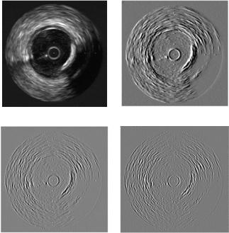
Figure 2.7: Local binary pattern response. (a) Original image. (b) Local binary pattern output with parameters R = 3, P = 24.

0/1, 1/0 while we move over the neighborhood:

P−1

U (LBPP,R) = |s(gP−1 − gc) − s(g0 − gc)| + |s(gp − gc) − s(gp−1 − gc)|

p=1

Therefore,

Figure 2.7 shows an example of an IVUS image filtered using a uniform rotation invariant local binary pattern with values P = 24, R = 3. The feature extraction image displayed in the figure looks like a discrete response focussed on the structure shape and homogeneity.

2.2.2 Analytic Kernel-Based Methods

2.2.2.1 Derivatives of Gaussian

In order to handle image structures at different scales in a consistent manner, a linear scale-space representation is proposed in [24, 34]. The basic idea is to embed the original signal into an one-parameter family of gradually smoothed signals, in which fine scale details are successively suppressed. It can be shown that the Gaussian kernel and its derivatives are one of the possible smoothing kernels for such scale-space. The Gaussian; kernel is well-suited for defining a space-scale because of its linearity and spatial shift invariance, and the notion

that structures at coarse scales should be related to structures at finer scales in a well-behaved manner (new structures are not created by the smoothing method). Scale-space representation is a special type of multiscale representation that comprises a continuous scale parameter and preserves the same spatial sampling at all scales. Formally, the linear-space representation of a continuous signal is constructed as follows. Let f : N → represent any given signal. Then, the scale-space representation L : N × R+ → is defined by L(·; 0) = f so that

L(·; t) = g(·; t) f

where t + is the scale parameter, and g : N xR+{0} → is the Gaussian kernel. In arbitrary dimensions, it is written as:

The square root of the scale parameter, σ = √(t), is the standard deviation of the kernel g and is a natural measure of spatial scale in the smoothed signal at scale t. From this scale-space representation, multiscale spatial derivatives can be defined by

Lx n (·; t) = ∂x n L(·; t) = gx n (·; t) f,

where gx n denotes a derivative of some order n.

The main idea behind the construction of this scale-space representation is that the fine scale information should be suppressed with increasing values of the scale parameter. Intuitively, when convolving a signal by a Gaussian kernel with standard deviation σ = √t, the effect of this operation is to suppress most of the structures in the signal with a characteristic length less than

σ . Different directional derivatives can be used to extract different kind of structural features at different scales. It is shown in the literature [35] that a possible complete set of directional derivatives up to the third order are ∂n = [∂0, ∂90, ∂02, ∂602 , ∂1202 , ∂03, ∂453 , ∂903 , ∂1353 ]. So our feature vector will consist on the directional derivatives, including the zero derivative, for each of the n scales desired:

F = {{∂n, Gn}, n }

The wavelet transform of f at scale s and position u is computed by correlating

The continuous wavelet transform W f (u, s) is a two-dimensional representation of a one-dimensional signal f . This indicates the existence of some redundancy that can be reduced and even removed by subsampling the parameters of these transforms. Completely eliminating the redundancy is equivalent to building a basis of the signal space.

The decomposition of a signal gives a series of coefficients representing the signal in terms of the base from a mother wavelet, that is, the projection of the

signal on the space formed by the base functions.

The continuous wavelet transform has two major drawbacks: the first, stated formerly, is redundancy and the second, impossibility to calculate it unless a discrete version is used. A way to discretize the dilation parameter is a = a0m, m Z, a0 = 1 constant. Thus, we get a series of wavelets ψm of width, a0m. Usually, we take a0 > 1, although it is not important because m can be positive or negative. Often, a value of a0 = 2 is taken. For m = 0, we make s to be the only integer multiples of a new constant s0. This constant is chosen in such a way that the translations of the mother wavelet, ψ (t − ns0), are as close as possible in order

to cover the whole real line. Then, the election of s level is as follows:

that covers the entire real axis as well as the translations ψ (t − ns0) does. Summarizing, the discrete wavelet transform consists of two discretizations in the transformation Eq. (2.1),

a = a0m, b = nb0a0m, m, n Z, a0 > 1, b0 > 0

The multiresolution analysis (MRA) tries to build orthonormal bases for a dyadic grid, where a0 = 2, b0 = 1, which besides have a compact support region. Finally, we can imagine the coefficients dm,n of the discrete wavelet transform as the sampling of the convolution of signal f (t) with different filters ψm(−t),

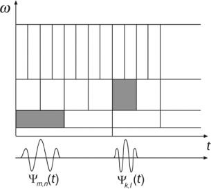
Figure 2.9: Scale-frequency domain of wavelets.

where ψm(t) = a0−m/2ψ (a−mt)

Figure 2.9 shows the dual effect of shrinking of the mother wavelet as the frequency increases, and the translation value decreasing as the frequency increases. The mother wavelet keeps its shape but if high-frequency analysis is desired the spatial support of the wavelet has to decrease. On the other hand, if the whole real line has to be covered by translations of the mother wavelet, as the spatial support of the wavelet decreases, the number of translations needed to cover the real line increases. Unlike Fourier transform, where translations of analysis are at the same distance for all the frequencies.

The choice of a representation of the wavelet transform leads us to define the concept of a frame. A frame is a complete set of functions that, though able to span L2( ), is not a base because it lacks the property of linear independence. MRA proposed in [26] is another representation in which the signal is decomposed in an approximation at a certain level L with L detail terms of higher resolutions. The representation is an orthonormal decomposition instead of a redundant frame, and therefore, the number of samples that defines a signal is the same as that the number of coefficients of their transform. A MRA consists

of a sequence of function subspaces of successive approximation. Let Pj be an operator defined as the orthonormal projection of functions of L2 over the space Vj . The projection of a function f over Vj is a new function that can be expressed as a linear combination of the functions that form the orthonormal base of Vj . Coefficients of the combination of each base function is the scalar product of f with the base functions:

Earlier we have pointed out the nesting condition of the Vj spaces, Vj Vj−1. Now, if f Vj−1 then f Vj or f is orthonormal to all the Vj functions, that is, we divide Vj−1 in two disjoint parts: Vj and other space W j , such that if f Vj , g W j , f g; W j is the orthonormal complement of Vj in Vj−1:

Vj−1 = Vj W j

where symbol measures the addition of orthonormal spaces. Applying the former equation and the completeness condition, then

· · · W j−2 W j−1 W j W j+1 · · · = W j = L2

j Z

So, we can write

Pj−1 f = Pj f + f, ψ j,n ψ j,n n Z

From these equations some conclusions can be extracted. First, the projection of a signal f in a space Vj gives a new signal Pj f , an approximation of the initial signal. Secondly, we have a hierarchy of spaces, then Pj−1 f will be a better approximation (more reliable) than Pj f . Since Vj−1 can be divided in two subspaces Vj and W j , if Vj is an approximation space then W j , which is the complementary orthonormal space, it is the detail space. The less the j, the finer the details.

Vj = Vj+1 W j+1 = Vj+2 W j+2 = · · ·

=VL WL WL−1 · · · W j+1

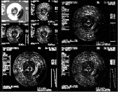
Figure 2.10: Wavelets multiresolution decomposition.

This can be viewed as a decomposition tree (see Fig. 2.10). At the top-left side of the image the approximation can be seen, and surrounding it the successive details. The further the detail is located the finer the information provided. So, the details at the bottom and at the right side of the image have information about the finer details and the smallest structures of the image decomposed. Therefore, we have a feature vector composed by the different detail approaches and the approximation for each of the pixels.

2.2.2.3 Gabor Filters

Gabor filters represent another multiresolution technique that relies on scale and direction of the contours [25, 37]. The Gabor filter consists of a two-dimensional sinusoidal plane wave of a certain orientation and frequency that is modulated in amplitude by a two-dimensional Gaussian envelope. The spatial representation of the Gabor filter is as follows:

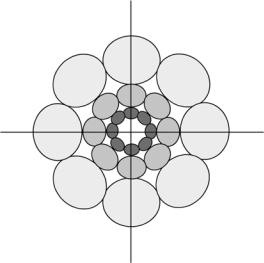
Figure 2.11: The filter set in the spatial-frequency domain.

where u0 and φ are the frequency and phase of the sinusoidal plane wave along the x axis and σx and σy are the space constants of the Gaussian envelope along the x and y axis, respectively. Filters at different orientations can be created by rigid rotation of x–y coordinate system.

An interesting property of this kind of filters is their frequency and orientation-selection. This fact is better displayed in the frequency domain. Figure 2.11 shows the filter area in the frequency domain. We can observe that each of the filters has a certain domain defined by each of the leaves of the Gabor “rose.” Thus, each filter responds to a certain orientation and at a certain detail level. Wider the range of orientations, smaller the space filter dimensions and smaller the details captured by the filter, as bandwidth in the frequency domain is inversely related to filter scope in the space domain. Therefore, Gabor filters provide a trade-off between localization or resolution in both the spatial and the spatial-frequential domains. As it has been mentioned, different filters emerge from rotating the x–y coordinate system. For practical approaches one can use four angles θ0 = 0◦, 45◦, 90◦, 135◦. For an image array of N pixels (with N power of 2), the following values of u0 are suggested [25, 37]:

cycles per image width. Therefore, the orientations and bandwidth of such filters vary with 45◦ and 1 octave. These parameters are chosen because there is physiologic evidences of frequency bandwidth of simple cells in visual cortex being of about 1 octave, and Gabor filters try to mimic part of the human perceptual system.

The Gabor function is an approximation to a wavelet. However, though admissible, it does not result in an orthogonal decomposition, and therefore, a transformation based on Gabor’s filters is redundant. On the other hand, Gabor filtering is designed to be nearly orthogonal, reducing the amount of overlap between filters.

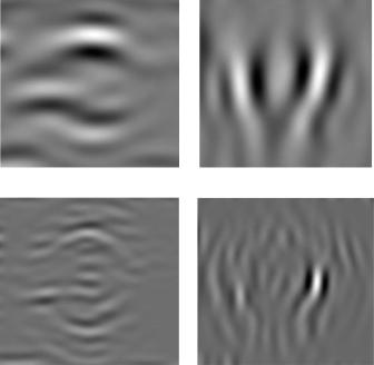
Figure 2.12 shows different responses for different filters of the spectrum. Figures 2.12(a) and 2.12(b) correspond to the inner filters with reduced frequency bandwidth displayed in Fig. 2.11. It can be seen that they deliver only

Figure 2.12: Gabor filter bank example responses. (a) Gabor vertical energy of a coarse filter response. (b) Gabor horizontal energy of a coarse filter response.

(c) Gabor vertical energy of a detail filter response. (d) Gabor horizontal energy of a detail filter response.

Table 2.1: Dimensionality of the feature space

provided by the texture feature extraction process

coarse information of the structure and the borders are far from the original location. In the same way, Figs. 12(c) and 12(d) are filters located on a further ring, and therefore respond to details in the image.

It can be observed that the feature extraction process is a transformation of the original two-dimensional image domain to a feature space that probably will have different dimensions. In some cases, the feature space remains low, as in fractal dimension and local binary patterns, that with very few features try to describe the texture present in the image. However, several feature spaces require higher dimensions, such as accumulation local moments, co-occurrence matrix measures, or derivatives of Gaussian. Table 2.1 shows the dimensionality of the different spaces generated by the feature extraction process in our texturebased IVUS analysis.

The next step after the feature extraction is the classification process. As a result of the disparity of the dimensionality of the feature spaces, we have to choose a classification scheme that is able to deal with high dimensionality feature data.

2.3 Classification Process

Once completed the feature extraction process, we have a set of features disposed in feature vectors. Each feature vector is composed of all the feature measures computed at each pixel. Therefore, for each pixel we have an n-dimensional point in the feature space, where n is the number of features. This set of data is the input to the classification process. The classification process