

Kluwer - Handbook of Biomedical Image Analysis Vol
.2.pdf10 |
Leemput et al. |
Figure 1.4: Top row (from left to right): Original T1 MPRAGE patient image; CSF segmented by atlas-guided intensity-based tissue classification using affine registration to atlas template; CSF segmented after nonrigid matching of the atlas. Middle row: Atlas priors for gray matter, white matter, and CSF affinely matched to patient image. Bottom row: Idem after nonrigid matching.
segmentation process, which alternates between pixel classification and parameter estimation, converges to the correct segmentation solution (Fig. 1.4 (top row, middle)). Nonrigid registration of atlas and patient images using the method presented in [24] can better cope with this extra variability. Note how the segmentation of the enlarged ventricles is much improved (see Fig. 1.4 (top row, right)).
1.1.4 Model-Based Brain Tissue Classification: Overview
The standard intensity model described in section 1.1.2 can be extended in several ways in order to better represent real MR images of the brain. The overall
Model-Based Brain Tissue Classification |
11 |
strategy is to build increasingly better statistical models for normal brain MR images and to detect disease-related (e.g. MS or CJD) signal abnormalities as voxels that cannot be well explained by the model. Figure 1.5 shows typical samples of the proposed models in increasing order of complexity, starting from the original mixture model, shown in Fig. 1.5(a). For each of the models, the same EM framework is applied to estimate the model parameters. An unusual aspect of the methods presented here is that all model parameters are estimated from the data itself, starting from an initialization that is obtained without user intervention. This ensures that the models retrain themselves fully automatically on each individual scan, allowing the method to analyze images with previously unseen MR pulse sequences and voxel sizes. In this way, subjective manual tuning and training is eliminated, which would make the results not fully reproducible.
The first problem for the segmentation technique of section 1.1.2 is the corruption of MR images with a smoothly varying intensity inhomogeneity or bias field [25, 26], which results in a nonuniform intensity of the tissues over the image area as shown in Fig. 1.6. This bias is inherent to MR imaging and is caused by equipment limitations and patient-induced electrodynamic interactions [26]. Although not always visible for a human observer, it can cause serious misclassifications when intensity-based segmentation techniques are used. In section 1.2 the mixture model is therefore extended by explicitly including a parametric model for the bias field. Figure 1.5(b) shows a typical sample of the resulting model. The model parameters are then iteratively estimated by interleaving three steps: classification of the voxels; estimation of the normal distributions; and estimation of the bias field. The algorithm is initialized with information from a digital brain atlas about the a priori expected location of tissue classes. This allows full automation of the method without need for user interaction, yielding fully objective and reproducible results.
As a consequence of the assumption that the tissue type of each voxel is independent from the tissue type of the other voxels, each voxel is classified independently, based only on its intensity. However, the intensity of some tissues surrounding the brain is often very similar to that of brain tissue, which makes a correct classification based on intensity alone impossible. Therefore, the model is further extended in section 1.3 by introducing a Markov random field (MRF) prior on the underlying tissue labels of the voxels. Such a MRF takes into account that the various tissues in brain MR images are not just randomly distributed over the image area, but occur in clustered regions of homogeneous tissue. This
12 |
Leemput et al. |
(a) |
(b) |
(c) |
(d) |
(e)
Figure 1.5: Illustration of the statistical models for brain MR images used in this study. The mixture model (a) is first extended with an explicit parametric model for the MR bias field (b). Subsequently, an improved spatial model is used that takes into account that tissues occur in clustered regions in the images
(c). Then the presence of pathological tissues, which are not included in the statistical model, is considered (d). Finally, a downsampling step introduces partial voluming in the model (e).
Model-Based Brain Tissue Classification |
13 |
is illustrated in Fig. 1.5(c), which shows a sample of the total resulting image model. The MRF brings general spatial and anatomical constraints into account during the classification, facilitating discrimination between tissue types with similar intensities such as brain and nonbrain tissues.
The method is further extended in section 1.4 in order to quantify lesions or disease-related signal abnormalities in the images (see Fig. 1.5(d)). Adding an explicit model for the pathological tissues is difficult because of the wide variety of their appearance in MR images, and because not every individual scan contains sufficient pathology for estimating the model parameters. These problems are circumvented by detecting lesions as voxels that are not well explained by the statistical model for normal brain MR images. Based on principles borrowed from the robust statistics literature, tissue-specific voxel weights are introduced that reflect the typicality of the voxels in each tissue type. Inclusion of these weights results in a robustized algorithm that simultaneously detects lesions as model outliers and excludes these outliers from the model parameter estimation. In section 1.5, this outlier detection scheme is applied for fully automatic segmentation of MS lesions from brain MR scans. The method is validated by comparing the automatic lesions segmentations to manual tracings by human experts.
Thus far, the intensity model assumes that each voxel belongs to one single tissue type. Because of the complex shape of the brain and the finite resolution of the images, a large part of the voxels lies on the border between two or more tissue types. Such border voxels are commonly referred to as partial volume (PV) voxels as they contain a mixture of several tissues at the same time. In order to be able to accurately segment major tissue classes as well as to detect the subtle signal abnormalities in MS, e.g., the model for normal brain MR images can be further refined by explicitly taking this PV effect into account. This is accomplished by introducing a downsampling step in the image model, adding up the contribution of a number of underlying subvoxels to form the intensity of a voxel. In voxels where not all subvoxels belong to the same tissue type, this causes partial voluming, as can be seen in Fig. 1.5(e). The derived EM algorithm for estimating the model parameters provides a general framework for partial volume segmentation that encompasses and extends existing techniques. A full presentation of this PV model is outside the scope of this chapter, however. The reader is referred to [27] for further details.
14 |
Leemput et al. |
(a) |
(b) |
Figure 1.6: The MR bias field in a proton density-weighted image. (a) Two axial
slices; (b) the same slices after intensity thresholding.
1.2 Automated Bias Field Correction
A major problem for automated MR image segmentation is the corruption with a smoothly varying intensity inhomogeneity or bias field [25, 26]. This bias is inherent to MR imaging and is caused by equipment limitations and patient-induced electrodynamic interactions. Although not always visible for a human observer, as illustrated in Fig. 1.6, correcting the image intensities for bias field inhomogeneity is a necessary requirement for robust intensity-based image analysis techniques. Early methods for bias field estimation and correction used phantoms to empirically measure the bias field inhomogeneity [28]. However, this approach assumes that the bias field is patient independent, which it is not [26]. Furthermore, it is required that the phantom’s scan parameters are the same as the patient’s, making this technique impractical and even useless as a retrospective bias correction method. In a similar vein, bias correction methods have been proposed for surface coil MR imaging using an analytic correction of the MR antenna reception profile [29], but these suffer from the same drawbacks as do the phantom-based methods. Another approach, using homomorphic filtering [30], assumes that the frequency spectrum of the bias field and the image structures are well separated, but this assumption is generally not valid for MR images [28, 31].
While bias field correction is needed for good segmentation, many approaches have exploited the idea that a good segmentation helps to estimate the bias field. Dawant et al. [31] manually selected some points inside white matter and estimated the bias field as the least-squares spline fit to the
Model-Based Brain Tissue Classification |
15 |
intensities of these points. They also presented a slightly different version where the reference points are obtained by an intermediate classification operation, using the estimated bias field for final classification. Meyer et al. [32] also estimated the bias field from an intermediate segmentation, but they allowed a region of the same tissue type to be broken up into several subregions which creates additional but sometimes undesired degrees of freedom.
Wells et al. [4] described an iterative method that interleaves classification with bias field correction based on ML parameter estimation using an EM algorithm. However, for each set of similar scans to be processed, their method, as well as its refinement by other authors [5, 6], needs to be supplied with specific tissue class conditional intensity models. Such models are typically constructed by manually selecting representative points of each of the classes considered, which may result in segmentations that are not fully objective and reproducible.
In contrast, the method presented here (and in [23]) does not require such a preceding training phase. Instead, a digital brain atlas is used with a priori probability maps for each tissue class to automatically construct intensity models for each individual scan being processed. This results in a fully automated algorithm that interleaves classification, bias field estimation, and estimation of class-conditional intensity distribution parameters.
1.2.1 Image Model and Parameter Estimation
The mixture model outlined in section 1.1.2 is extended to include a model for the bias field. We model the spatially smoothly varying bias fields as a linear combination of P polynomial basis functions φp(xj ), p = 1, 2, . . . , P, where xj denotes the spatial position of voxel j. Not the observed intensities yj but the bias corrected intensities uj are now assumed to be distributed according to a mixture of class-specific normal distributions, such that Eq. (1.1) above is replaced by
f (yj | l j , ) = GΣl j (uj − µl j )
uj = yj − [b1 · · · bC ]t
φ1(xj )
.
.
.
φP (xj )

16 |
Leemput et al. |
with bc, c = 1, 2, . . . , C indicating the bias field parameters of MR channel c, and = {µk, Σk, bc, k = 1, 2, . . . , K, c = 1, 2, . . . , C} as the total set of model parameters.
With the addition of the bias field model, estimation of the model parameters with an EM algorithm results in an iterative procedure that now interleaves three steps (see Fig. 1.7): classification of the image voxels (Eq. 1.4); estimation of the normal distributions (Eqs. (1.5) and (1.6) but with the bias corrected intensities uj replacing the original intensities yj ); and estimation of the bias field. For the unispectral case, the bias field parameters are given by the following expression3:
b(m) = ( At W(m) A)−1 At W(m) R(m)
with
A |
|
φ1 |
(x2) φ2 |
(x2) φ3 |
(x2) |
· · · |
|||||
|
|
φ1 |
(x1) |
φ2 |
(x1) |
φ3 |
(x1) |
|
|
. |
|
|
|
. |
|
. |
|
. |
|
|
|||
|
= |
|
|
|
|
|
|
· · · |
|||
|
. |
|
. |
|
. |
|
|
|
|
||
|
|
|
|
. |
. |
|
|
||||
|
|
|
. |
|
. |
|
. |
|
|
|
|
W(m) = diag w j |
(m), |
|
||||
|
|
y2 |
|
(m) |
|
|
R(m) |
|
|
y˜2(m) |
, |
||
|
|
y1 |
− y˜1 |
|
||
|
|
|
. |
|
|
|
|
= |
|
− |
|
|
|
|
. |
|
|
|||
|
|
|
|
|
|
|
.
j |
|
= |
k |
jk |
, |
jk |
= |
|
σk2 |
|
w(m) |
|
w(m) |
w(m) |
|
f l j = k | Y, (m−1) |
|
||||
|
y˜ j |
= |
|
k w(jkm) |
|
|
|
|
||
|
|
(m) |
|
k w(jkm) |
µk(m) |
|
|
|
|
|
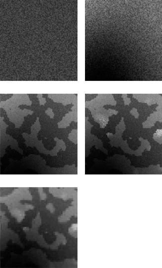
This can be interpreted as follows (see Fig. 1.8). Based on the current classification and distribution estimation, a prediction {y˜ j , j = 1, 2, . . . , J} of the MR image without the bias field is constructed (Fig. 1.8(b)). A residue image R (Fig. 1.8(c)) is obtained by subtracting this predicted signal from the original image (Fig. 1.8(a)). The bias (Fig. 1.8(e)) is then estimated as a weighted least-squares fit through the residue image using the weights W (Fig. 1.8(d)), each voxel’s weight being inversely proportional to the variance of the class that voxel belongs to. As can be seen from Fig. 1.8(d), the bias field is therefore computed primarily from voxels that belong to classes with a narrow intensity distribution, such as white and gray matter. The smooth spatial model extrapolates the bias
3 For more general expressions for the multispectral case we refer to [23]; in the unispectral case yj = yj , µk = µk, and Σk = σk2 .

Model-Based Brain Tissue Classification |
17 |
update bias field
classify
update mixture model
Figure 1.7: Adding a model for the bias field results in a three-step expectationmaximization algorithm that iteratively interleaves classification, estimation of the normal distributions, and bias field correction.
(a) |
(b) |
(c) |
(d) |
(e) |
(f) |
Figure 1.8: Illustration of the bias correction step on a 2D slice of a T1-weighted MR image: (a) original image; (b) predicted signal based on previous iterations;
(c) residue image; (d) weights; (e) estimated bias field; (f) corrected image. (Source: Ref. [23].)

18 |
Leemput et al. |
field from these regions, where it can be confidently estimated from the data, to regions where such estimate is ill-conditioned (CSF, nonbrain tissues).
1.2.2 Examples and Discussion
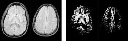
Examples of the performance of the method are shown in Figs. 1.9 and 1.10. Figure 1.9 depicts the classification of a high-resolution sagittal T1-weighted MR image, both for the original two-step algorithm without bias correction of section 1.1.2 and for the new three-step algorithm with bias correction. Because a relatively strong bias field reduces the intensities at the top of the head, bias correction is necessary as white matter is wrongly classified as gray matter in that area otherwise. Figure 1.10 clearly shows the efficiency of the bias correction on a 2-D multislice T1-weighted image. Such multislice images are acquired in an interleaved way, and are typically corrupted with a slice-by-slice constant intensity offset, commonly attributed to gradient eddy currents and crosstalk
(a)
(b)
(c)
(d)
Figure 1.9: Slices of a high-resolution T1-weighted MR image illustrating the performance of the method: (a) original data; (b) white matter classification without bias correction; (c) white matter classification with bias correction;
(d) estimated bias field. (Source: Ref. [23].)

Model-Based Brain Tissue Classification |
19 |
Figure 1.10: An example of bias correction of a T1-weighted 2-D multislice image corrupted with slice-by-slice offsets. From top row to bottom row: original data, estimated bias, corrected data. (Source: Ref. [23].)
between slices [25], and clearly visible as an interleaved bright-dark intensity pattern in a cross-section orthogonal to the slices in Fig. 1.10.
In earlier EM approaches for bias correction, the class-specific intensity distribution parameters µk and Σk were determined by manual training and kept fixed during the iterations [4–6]. It has been reported [6, 33, 34] that these methods are sensitive to the training of the classifier, i.e., they produce different results depending on which voxels were selected for training. In contrast, our algorithm estimates its tissue-specific intensity distributions fully automatically on each individual scan being processed, starting from a digital brain atlas. This avoids all manual intervention, yielding fully objective and reproducible results. Moreover, it eliminates the danger of overlooking some tissue types during a manual training phase, which is typically a problem in regions surrounding the