

Kluwer - Handbook of Biomedical Image Analysis Vol
.2.pdfSupervised Texture Classification for Intravascular Tissue Characterization |
61 |
this category, we can find clustering methods for unsupervised classification and, for supervised classification, methods like maximum likelihood, nearest neighbors, etc.
The following sections are devoted to describe the following: First, the most significative texture methods used in the literature. Secondly, some of the most successful classification methods applied to IVUS characterization are reviewed. Third, we describe the result of using such techniques for tissue characterization and conclude about the optimal feature space to describe tissue plaque and the best classifier to discriminate it.
2.2 Feature Spaces
Gray-level thresholding is not enough for robust tissue characterization. Therefore, it is generally approached as a texture discrimination problem. This line of work is a classical extension of previous works on biological characterization, which also relies on texture features as has been mentioned in the former section. The co-occurrence matrix is the most favored and well known of the texture feature extraction methods due to its discriminative power in this particular problem but it is not the only one nor the fastest method available. In this section, we make a review of different texture methods that can be applied to the problem in particular, from the co-occurrence matrix measures method to the most recent texture feature extractor, local binary patterns.
To illustrate the texture feature extraction process we have selected a set of techniques basing our criterion of selection on the most widespread methods for tissue characterization and the most discriminative feature extractors reported in the literature [21].
Basically, the different methods of feature extraction emphasize on different fundamental properties of the texture such as scale, statistics, or structure. In this way, under the nonelemental statistics property we can find two well-known techniques, co-occurrence methods [22] and higher order statistics represented by moments [23]. Under the label of scale property we should mention methods such as derivatives of Gaussian [24], Gabor filters [25], or wavelet techniques [26]. Regarding structure-related measures there are methods such as fractal dimension [27] and local binary patterns [28].
62 |
Pujol and Radeva |
To introduce the texture feature extraction methods we divide them into two groups: The first group, that forms the statistic-related methods, is comprised of co-occurrence matrix measures, accumulation local moments, fractal dimension, and local binary patterns. All these methods are somehow related to statistics. Co-occurrence matrix measures are second-order measures associated to the probability density function estimation provided by the co-occurrence matrix. Accumulation local moments are directly related to statistics. Fractal dimension is an approximation of the roughness of a texture. Local binary patterns provides a measure of the local inhomogeneity based on an “averaging” process. The second group, that forms the analytic kernel-based extraction techniques, comprises Gabor bank of filters, derivatives of Gaussian filters, and wavelet decomposition. The last three methods are derived from analytic functions and sampled to form a set of filters, each focused on the extraction of a certain feature.
2.2.1 Statistic-Related Methods
2.2.1.1 Co-occurrence Matrix Approach
In 1962 Julesz [29] showed the importance of texture segregation using secondorder statistics. Since then, different tools have been used to exploit this issue. The gray-level co-occurrence matrix is a well-known statistical tool for extracting second-order texture information from images [22]. In the co-occurrence method, the relative frequencies of gray-level pairs of pixels at certain relative displacement are computed and sorted in a matrix, the co-occurrence matrix
P. The co-occurrence matrix can be thought of as an estimate of the joint probability density function of gray-level pairs in an image. For G gray levels in the image, P will be of size G × G. If G is large, the number of pixel pairs contributing to each element, pi, j in P is low, and the statistical significance poor. On the other hand, if the number of gray levels is low, much of the texture information may be lost in the image quantization. The element values in the matrix, when normalized, are bounded by [0, 1], and the sum of all element values is equal to 1.
P(i, j, D, θ ) = P(I(l, m) = i and I(l + D cos(θ ), m + D sin(θ )) = j
where I(l, m) is the image at pixel (l, m), D is the distance between pixels,
Supervised Texture Classification for Intravascular Tissue Characterization |
63 |
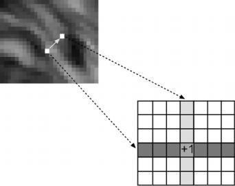
Figure 2.2: Co-occurrence matrix explanation diagram (see text).
and θ is the angle. It has been proved by other researchers [21, 30] that the nearest neighbor pairs at distance D at orientations θ = {0◦, 45◦, 90◦, 135◦} are the minimum set needed to describe the texture second-order statistic measures. Figure 2.2 illustrates the method providing a graphical explanation. The main idea is to create a “histogram” of the occurrences of having two pixels of certain gray levels at a determined distance with a fixed angle. Practically, we add one to the cell of the matrix pointed by the gray levels of two pixels (one pixel gray level gives the file and the other the column of the matrix) that fulfill the requirement of being at a certain predefined distance and angle.
Once the matrix is computed several characterizing measures are extracted. Many of these features are derived by weighting each of the matrix element values and then summing these weighted values to form the feature value. The weight applied to each element is based on a feature-weighing function, so by varying this function, different texture information can be extracted from the matrix. We present here some of the most important measures that characterize the co-occurrence matrices: energy, entropy, inverse difference moment, shade, inertia, and promenance [30]. Let us introduce some notation for the definition of the features:
64 |
|
|
|
Pujol and Radeva |
P(i, j) is the (i, j)th element of a normalized co-occurrence matrix |
||||
Px(i) = j |
P(i, j) |
|
|
|
Py( j) = i |
P(i, j) |
|
|
|
µx = i |
i j |
P(i, j) = i |
iPx(i) = E{i} |
|
µy = j |
j i |
P(i, j) = j |
j Py( j) = E{ j} |
|
With the above notation, the features can be written as follows:
Energy = |
i, j |
P(i, j)2 |
|||
Entropy = − i, j |
P(i, j) log P(i, j) |
||||
Inverse difference moment = i, j |
|
|
1 |
P(i, j) |
|
|
1 + (i − j)2 |
||||
Shade = i, j |
(i + j − µx − µy)3 P(i, j) |
||||
Inertia = i, j |
(i − j)2 P(i, j) |
||||
Promenance = i, j |
(i + j − µx − µy)4 P(i, j) |
||||
Hence, we create a feature vector for each of the pixels by assigning each feature measure to a component of the feature vector. Given that we have four different orientations and the six measures for each orientation, the feature vector is a 24-dimensional vector for each pixel and for each distance. Since we have used two distances D = 2 and D = 3, the final vector is a 48-dimensional vector.
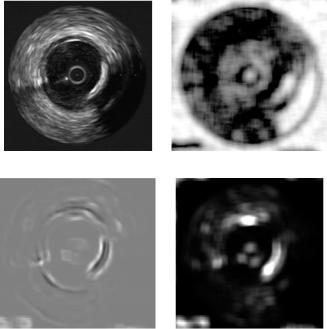
Figure 2.3 shows responses for different measures on the co-occurrence matrices. Although a straightforward interpretation of the feature extraction response is not easy, some deduction can be made by observing the figures. Figure 2.3(b) shows shade measure; as its name indicates it is related to the shadowed areas in the image, and thus, localizing the shadowing behind the calcium plaque. Figure 2.3(c) shows inverse different moment response, this measure seems to be related to the first derivative of the image, enhancing contours. Figure 2.3(d) depicts the output for the inertia measure, which seems to have some relationship with local homogeneity of the image.
Supervised Texture Classification for Intravascular Tissue Characterization |
65 |
(a) |
(b) |
(c) |
(d) |
Figure 2.3: Response of an IVUS image to different measures of the cooccurrence matrix. (a) Original image, (b) measure shade response, (c) inverse different moment, and (d) inertia.
2.2.1.2 Accumulation Local Moments
Geometric moments have been used effectively for texture segmentation in many different application domains [23]. In addition, other kind of moments have been proposed: Zernique moments, Legendre moments, etc. By definition, any set of parameters obtained by projecting an image onto a two-dimensional polynomial basis is called moments. Then, since different sets of polynomials up to the same order define the same subspace, any complete set of moments up to given order can be obtained from any other set of moments up to the same order. The computation of some of these sets of moments leads to very long processing times, so in this section a particular fast computed moment set has been chosen. This set of moments is known as the accumulation local moments. Two kind of accumulation local moments can be computed, direct accumulation and reverse accumulation. Since direct accumulation is more sensitive to round
66 Pujol and Radeva
off errors and small perturbations in the input data [31], the reverse accumulation moments are recommendable.
The reverse accumulation moment of order (k − 1, l − 1) of matrix Iab is the value of Iab[1, 1] after bottom-up accumulating its column k times (i.e., after applying k times the assignment Iab[a − i, j] ← Iab[a − i, j] + Iab[a − i + 1, j], for i = 0 to a − 1, and for j = 1 to b), and accumulating the resulting first row from right to left l times (i.e., after applying l times the assignment Iab[1, b − j] ←
Iab[1, b − j] + Iab[1, b − j + 1], for j = 1 to b − 1). The reverse accumulation moment matrix is defined so that Rmn[k.l] is the reverse accumulation moment of order (k − 1, l − 1).
Consider the matrix in the following example:
|
0 |
1 |
2 |
|
4 |
2 |
3 |
||
|
1 |
1 |
1 |
|
|
|
|
According to the definition, its reverse accumulation moment of order (1,2) requires two column accumulations,
|
|
5 |
3 |
4 |
|
|
|
9 |
5 |
|
7 |
|
|
|
|
5 |
4 |
6 |
|
→ |
14 |
9 |
|
13 |
|
|
|
|
4 |
2 |
3 |
|
4 |
2 |
3 |
|
|||||
|
|
|
|
|
|
|
|
|
|
|
|
|
|
and three right to left accumulations of the first row: |
|
|
|||||||||||
|
36 22 13 → |
71 |
35 |
13 |
→ |
119 48 13 |
|||||||
Then it is said that the reverse accumulation moment of order (1,2) of the former matrix is 119.
The set of moments alone is not sufficient to obtain good texture features in certain images. Some iso-second order texture pairs, which are preattentively discriminable by humans, would have the same average energy over finite regions. However, their distribution would be different for the different textures. One solution suggested by Caelli is to introduce a nonlinear transducer that maps moments to texture features [32]. Several functions have been proposed in the literature: logistic, sigmoidal, power function, or absolute deviation of feature vectors from the mean [23]. The function we have chosen is the hyperbolic tangent function, which is logistic in shape. Using the accumulation moments
| − ¯ |
image Im and a nonlinear operator tanh(σ (Im Im) an “average” is performed
Supervised Texture Classification for Intravascular Tissue Characterization |
67 |
(a) |
(b) |
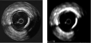
Figure 2.4: Accumulation local moments response. (a) Original image. (b) Accumulation local moment of order (3,1).
throughout the region of interest. The parameter σ controls the shape of the logistic function. Therefore each textural feature will be the result of the application of the nonlinear operator to the computed moments. If n = k · l moments are computed over the image, then the dimension of the feature vector will be n. Hence, a n-dimensional point is associated with each pixel of the image.
Figure 2.4 shows the response of moment (3,1) on an IVUS image. In this figure, the response seems to have a smoothing and enhancing effect, clearly resembling diffusion techniques.
2.2.1.3 Fractal Analysis
Another classic tool for texture description is the fractal analysis [13, 33], characterized by the fractal dimension. We talk roughly about fractal structures when a geometric shape can be subdivided in parts, each of which are approximately a reduced copy of the whole (this property is also referred as self-similarity). The introduction of fractals by Mandelbrot [27] allowed a characterization of complex structures that could not be described by a single measure using Euclidean geometry. This measure is the fractal dimension, which is related to the degree of irregularity of the surface texture.
The fractal structures can be divided into two subclasses: the deterministic fractals and the random fractals. Deterministic fractals are strictly self-similar, that is, they appear identical over a range of magnification scales. On the other hand, random fractals are statistical self-similar. The similarity between two scales of the fractal is ruled by a statistical relationship.

68 |
Pujol and Radeva |
The fractal dimension represents the disorder of an object. The higher the dimension, the more complex the object is. Contrary to the Euclidian dimension, the fractal dimension is not constrained to integer dimensions.
The concept of fractals can be easily extrapolated to image analysis if we consider the image as a three-dimensional surface in which the height at each point is given by the gray value of the pixel.
Different approaches have been proposed to compute the fractal dimension of an object. Herein we consider only three classical approaches: box-counting, Brownian motion, and Fourier analysis.
Box-Counting. The box-counting method is an approximation to the fractal dimension as it is conceptually related to self-similarity.
In this method the object to be evaluated is placed on a square mesh of various sizes, r. The number of mesh boxes, N, that contain any part of the fractal structure are counted.
It has been proved that in a self-similar structures there is a relationship between the reduction factor r and the number of divisions N into which the structure can be divided:
Nr D = 1
where D is the self-similarity dimension. Therefore, the fractal dimension can be easily written as
D = log N log 1/r
This process is done at various scales by altering the square size r. Therefore, the box-counting dimension is the slope of the regression line that better approximates the data on the plot produced by log N × log 1/r.
Fractal Dimension from Brownian Motion. The fractal dimension is found by considering the absolute intensity difference of pixel pairs, I( p1) −
I( p2), at different scales. It can be shown that for a fractal Brownian surface the following relationship must be satisfied:
E(|I( p1) − I( p2)|)α( (x2 − x1) + (y2 − y1))H
where E is the mean and H the Hurst coefficient. The fractal dimension is related to H in the following way: D = 3 − H. In the same way than the former
Supervised Texture Classification for Intravascular Tissue Characterization |
69 |
(a) |
(b) |
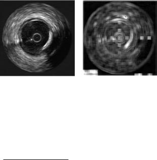
Figure 2.5: Fractal dimension from box-counting response. (a) Original image.
(b) Fractal dimension response with neighborhoods of 10 × 10.
method for calculating the fractal dimension the mean difference of intensities is calculated for different scales (each scale given by the euclidian distance
between two pixels), and the slope of the regression line between log E(|I( p1) −
√
I( p2)|) and (x2 − x1) + (y 2 − y1) gives the Hurst parameter.
Triangular Prism Surface Area Method. The triangular prism surface area (TPSA) algorithm considers an approximation of the “area” of the fractal structure using triangular prisms. If a rectangular neighborhood is defined by its vertices A, B, C, and D, the area of this neighborhood is calculated by tessellating the surface with four triangles defined for each consecutive vertex and the center of the neighborhood.
The area of all triangles for every central pixel is summed up to the entire area for different scales. The double logarithmic Richardson–Mandelbrot plot should again yield a linear line whose slope is used to determine the TPSA dimension. Figure 2.5 shows the fractal dimension value of each pixel of an IVUS image considering the fractal dimension of a neighborhood around the pixel. The size of the neighborhood is 10 × 10. The response of this technique seems to take into account the border information of the structures in the image.
2.2.1.4 Local Binary Patterns
Local binary patterns [28] are a feature extraction operator used for detecting “uniform” local binary patterns at circular neighborhoods of any quantization of
70 |
Pujol and Radeva |
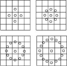
Figure 2.6: Typical neighbors: (Top left) P = 4, R = 1.0; (top right) P = 8,
R = 1.0; (bottom left) P = 12, R = 1.5; (bottom right) P = 16, R = 2.0.
the angular space and at any spatial resolution. The operator is derived based on a circularly symmetric neighbor set of P members on a circle of radius R. It is denoted by LBPriuP,R2. Parameter P controls the quantization of the angular space, and R determines the spatial resolution of the operator. Figure 2.6 shows typical neighborhood sets. To achieve gray-scale invariance, the gray value of the center pixel (gc) is subtracted from the gray values of the circularly symmetric neighborhood gp ( p = 0, 1, . . . , P − 1) and assigned a value of 1 if the difference is positive and 0 if negative.
1 if x ≥ 0
s(x) =
0otherwise
By assigning a binomial factor 2p for each value obtained, we transform the neighborhood into a single value. This value is the LBPR, P :
P
LBPR, P = s(gp − gc) · 2p
p=0
To achieve rotation invariance the pattern set is rotated as many times as necessary to achieve a maximal number of the most significant bits, starting always from the same pixel. The last stage of the operator consists on keeping the information of “uniform” patterns while filtering the rest. This is achieved using a transition count function U . U is a function that counts the number of transitions