

Kluwer - Handbook of Biomedical Image Analysis Vol
.2.pdf142 |
Wong |
from many objects (tissue TACs) and an improved SNR can be achieved [92]. It has been applied to segment a dynamic [11C]flumazenil PET data [92] and dynamic [123I]iodobenzamide SPECT images [93]. In the following, a clustering algorithm is described. Its application to automatic segmentation of dynamic FDG-PET data for tumor localization and detection is demonstrated in the next section. An illustration showing how to apply the algorithm to generate ROIs automatically for noninvasive extraction of physiological parameters will also be presented.
The segmentation method is based on cluster analysis. Our aim is to classify a number of tissue TACs according to their shape and magnitude into a smaller number of distinct characteristic classes that are mutually exclusive so that the tissue TACs within a cluster are similar to one another but are dissimilar to those drawn from other clusters. The clusters (or clustered ROIs) represent the locations in the images where the tissue TACs have similar kinetics. The kinetic curve associated with a cluster (i.e. cluster centroid) is the average of TACs in the cluster. Suppose that there exists k characteristic curves in the dynamic PET data matrix, X, which has M tissue TACs and N time frames with k M and that any tissue TAC belongs to only one of the k curves. The clustering algorithm then segments the dynamic PET data into k curves automatically based on a weighted least-squares distance measure, D, which is defined as
k |
M |
|
|
|
|
D{xi, µj } = |
xi − µj W2 |
(3.42) |
j=1 i=1
where xi RN is the ith tissue TAC in the data, µj RN is the centroid of cluster
C j , and W RN×N is a square matrix containing the weighting factors on the diagonal and zero for the off-diagonal entries. The weighting factors were used to boost the degree of separation between any TACs that have different uptake patterns but have similar least-squares distances to a given cluster centroid. They were chosen to be proportional to the scanning intervals of the experiment. Although this is not necessarily an optimal weighting, reasonably good clustering results can be achieved.
There is no explicit assumption on the structure of data and the clustering process proceeds automatically in an unsupervised manner. The minimal assumption for the clustering algorithm is that the dynamic PET data can be represented by a finite number of kinetics. As the number of clusters, k, for a given dataset is usually not known a priori, k is usually determined by trial and error.
Medical Image Segmentation |
143 |
In addition, the initial cluster centroid in each cluster is initialized randomly to ensure that all clusters are nonempty. Each tissue TAC is then allocated to its nearest cluster centroid according to the following criterion:
xl − µi 2W < xl − µj 2W
(3.43)
xl Ci i, j = 1, 2, . . . , k, i = j
where xl RN is the lth tissue TAC in X; µi RN and µj RN are the ith and jth cluster centroid, respectively; and Ci represents the ith cluster set. The centroids in the clusters are updated based on Eq. (3.43) so that Eq. (3.42) is minimized. The above allocation and updating processes are repeated for all tissue TACs until there is no reduction in moving a tissue TAC from one cluster to another. On convergence, the cluster centroids are mapped back to the original data space for all voxels. An improved SNR can be achieved because each voxel in the mapped data space is represented by one of the cluster centroids each of which possesses a higher statistical significance than an individual TAC.
Convergence to a global minimum is not always guaranteed because the final solution is not known a priori unless certain constraints are imposed on the solution that may not be feasible in practice. In addition, there may be several local minima in the solution space when the number of clusters is large. Restarting the algorithm with different initial cluster centroids is necessary to identify the best possible minimum in the solution space.
The algorithm is similar to the K -means type Euclidean clustering algorithm [40]. However, the K -means type Euclidean clustering algorithm requires that the data are normalized and it does not guarantee that the within-cluster cost is minimized since no testing is performed to check whether there is any cost reduction if an object is moved from one cluster to another.
3.6 Segmentation of Dynamic PET Images
The work presented in this section builds on our earlier research in which we applied the proposed clustering algorithm to tissue classification and segmentation of phantom data and a cohort of dynamic oncologic PET studies [94]. The study was motivated by our on-going work on a noninvasive modeling approach
144 |
Wong |
for quantification of FDG-PET studies where several ROIs of distinct kinetics are required [95, 96]. Manual delineation of ROIs restrain the reproducibility of the proposed modeling technique, and therefore, some other semiautomated and automated methods have been investigated and clustering appears as a promising alternative to automatically segment ROI of distinct kinetics. The results indicated that the kinetic and physiological parameters obtained with cluster analysis are similar to those obtained with manual ROI delineation, as we will see in the later sections.
3.6.1 Experimental Studies
3.6.1.1 Simulated [11C]Thymidine PET Study
To examine the validity of the segmentation scheme, we simulated a dynamic 2-[11C]thymidine (a marker of cell proliferation) PET study. 2-[11C]thymidine was chosen because it is being increasingly used in the research setting to evaluate cancer and treatment response, and it offers theoretical advantages over FDG such as greater specificity in the assessment of malignancy. Also, the kinetics are very similar for most tissues and the data are typically quite noisy. Thus, thymidine data represent a challenging example for testing the clustering algorithm.
Typical 2-[11C]thymidine kinetics for different tissues were derived from eight patients. The data were acquired on an ECAT 931 scanner (CTI/Siemens, Knoxville, TN). The dynamic PET data were acquired over 60 min with a typical sampling schedule (10 × 30 sec, 5 × 60 sec, 5 × 120 sec, 5 × 180 sec, 5 × 300 sec) and the tracer TAC in blood was measured with a radial artery catheter following tracer administration. Images were reconstructed using filtered back-projection (FBP) with a Hann filter cut-off at the Nyquist frequency. ROIs were drawn over the PET images to obtain tissue TACs in bone, bone marrow, blood pool, liver, skeletal muscle, spleen, stomach, and tumor. Impulse response functions (IRFs) corresponding to these tissues were determined by spectral analysis of the tissue TACs [97]. The average IRFs for each common tissue type were obtained by averaging the spectral coefficients across the subjects and convolved with a typical arterial input function, resulting in typical TACs for each tissue. The TACs were then assigned to the corresponding tissue types in a single slice of the Zubal phantom [98] which included blood vessels, bone, liver, bone marrow,
Medical Image Segmentation |
145 |
b
L |
T |
St |
|
||
|
|
BB
T M S
Mu
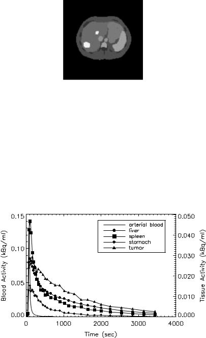
Figure 3.5: A slice of the Zubal phantom. B = blood vessels; b = bone; L = liver; M = marrow; Mu = muscle; S = spleen; St = stomach; T = tumor.
muscle, spleen, stomach, a large and small tumor in the liver (see Fig. 3.5). A dynamic sequence of sinograms was obtained by forward projecting the images into 3.13 mm bins on a 192 × 256 grid. Attenuation was included in the simulations for the purpose of obtaining the correct scaling of the noise. Poisson noise and blurring were added to simulate realistic sinograms. Noisy dynamic images were then reconstructed using FBP (Hann filter cut-off at the Nyquist frequency). Figure 3.6 shows the metabolite-corrected arterial blood curve and noisy 2-[11C]thymidine kinetics in some representative tissues.
Figure 3.6: Simulated noisy 2-[11C]thymidine kinetics in some representative regions. A metabolite-corrected arterial blood curve, which was used to simulate 2-[11C]thymidine kinetics in different tissues, is also shown.

146 |
Wong |
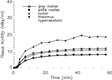
Figure 3.7: A slice of the Hoffman brain phantom. A tumor in white matter (white spot) and an adjacent hypometabolic region (shaded region) are shown.
3.6.1.2 Simulated FDG-PET Study
Dynamic FDG-PET study was simulated using a slice of the numerical Hoffman brain phantom [99] that modified using a template consisting of five different kinetics (gray matter, white matter, thalamus, tumor in white matter, and an adjacent hypometabolic region in left middle temporal gyrus), as shown in Fig. 3.7. The activities in gray matter and white matter were generated using a five-parameter three-compartment FDG model [100] with a measured arterial input function obtained from a patient (constant infusion of 400 MBq of FDG over 3 min). The kinetics present in the hypometabolic region, thalamus, and tumor were set to 0.7, 1.1, and 2.0 times the activity in gray matter. The kinetics were then assigned to each brain region and a dynamic sequence of sinograms (22 frames, 6 × 10 sec, 4 × 30 sec, 1 × 120 sec, 11 × 300 sec) was obtained by forward projecting the images into 3.13 mm bins on a 192 × 256 grid. Poisson noise and blurring were also added to simulate realistic sinograms. Dynamic images were reconstructed using FBP with Hann filter cut-off at the Nyquist frequency. The noisy FDG kinetics are shown in Fig. 3.8 and some of the kinetics are similar to each other due to the added noise and gaussian blurring, although their kinetics are different in the absence of noise and blurring. This is illustrated in the white matter and the hypometabolic region, and the gray matter and thalamus.
3.6.2 Cluster Validation
As mentioned earlier, the optimum number of clusters for a given dataset is usually not known a priori. It is advantageous if this number can be determined
Medical Image Segmentation |
147 |
||||||||||
|
|
|
|
|
|
|
|
|
|
|
|
|
|
|
|
|
|
|
|
|
|
|
|
|
|
|
|
|
|
|
|
|
|
|
|
|
|
|
|
|
|
|
|
|
|
|
|
|
|
|
|
|
|
|
|
|
|
|
|
|
|
|
|
|
|
|
|
|
|
|
|
|
|
|
|
|
|
|
|
|
|
|
|
|
|
|
|
|
|
|
|
|
|
|
|
|
|
|
|
|
|
|
|
|
|
|
|
|
|
|
|
|
|
|
|
|
|
|
|
|
|
|
|
|
|
|
|
|
|
|
|
Figure 3.8: Simulated noisy[18F]fluorodeoxyglucose (FDG) kinetics in different regions.
based on the given dataset. In this study, a model-based approach was adopted to cluster validation based on two information-theoretic criteria, namely, Akaike information criterion (AIC) [101] and Schwarz criterion (SC) [102], assuming that the data can be modeled by an appropriate probability distribution function (e.g. Gaussian). Both criteria determine the optimal model order by penalizing the use of a model that has a greater number of clusters. Thus, the number of clusters that yields the lowest value for AIC and/or SC is selected as the optimum. The use of AIC and SC has some advantages compared to other heuristic approaches such as the “bootstrap” resampling technique which requires a large amount of stochastic computation. This model-based approach is relatively flexible in evaluating the goodness-of-fit and a change in the probability model of the data does not require any change in the formulation except the modeling assumptions. It is noted, however, that both criteria may not indicate the same model as the optimum [102].
The validity of clusters is also assessed visually and by thresholding the average mean squared error (MSE) across clusters, which is defined as
1 |
k |
M |
|
|
|
|
|||
MSE = |
|
|
xi − µj W2 . |
(3.44) |
k |
|
|||
|
|
j=1 i=1 |
|
|
148 |
Wong |
Both approaches are subjective but they can provide an insight into the “correct” number of clusters.
3.6.3 Human Studies
The clustering algorithm has been applied to a range of FDG-PET studies and three examples (two patients with brain tumor and one patient with a lung cancer) are presented in this chapter. FDG-PET was chosen to assess the clustering algorithm because it is commonly used in clinical oncologic PET studies. All oncological PET studies were performed at the Department of PET and Nuclear Medicine, Royal Prince Alfred Hospital, Sydney, Australia. Ethical permissions were obtained from the Institutional Review Board.
Dynamic neurologic FDG-PET studies were performed on an ECAT 951R whole-body PET tomograph (CTI/Siemens, Knoxville, TN). Throughout the study the patient’s eyes were patched and ears were plugged. The patients received 400 MBq of FDG, infused at a constant rate over a 3-min period using an automated injection pump. At least 30 min prior to the study, patient’s hands and forearms were placed into hot water baths preheated to 44 ◦C to promote arterio-venous shunting. Blood samples were taken at approximately 30 sec for the first 6 min, and at approximately 8, 10, 15, 30, and 40 min, and at the end of emission data acquisition. A dynamic sequence of 22 frames was acquired for 60 min following radiotracer administration according to the following schedule: 6 × 10 sec, 4 × 30 sec, 1 × 2 min, 11 × 5 min. Data were attenuation corrected with a postinjection transmission method [103]. Images were reconstructed on a 128 × 128 matrix using FBP with a Shepp and Logan filter cut-off at 0.5 of the Nyquist frequency.
The dynamic lung FDG-PET study was commenced after intravenous injection of 487 MBq of FDG. Emission data were acquired on an ECAT 951R wholebody PET tomograph (CTI/Siemens, Knoxville, TN) over 60 min (22 frames, 6 × 10 sec, 4 × 30 sec, 1 × 2 min, and 11 × 5 min). Twenty one arterial blood samples were taken from the pulmonary artery using a Grandjean catheter to provide an input function for kinetic modeling.
The patient details are as follows:
Patient 1: The FDG-PET scan was done in a female patient, 6 months after resection of a malignant primary brain tumor in the right parieto-occipital
Medical Image Segmentation |
149 |
lobe. The scan was done to determine if there was evidence for tumor recurrence. A partly necrotic hypermetabolic lesion was found in the right parieto-occipital lobe that was consistent with tumor recurrence.
Patient 2: A 40-year-old woman had a glioma in the right mesial temporal lobe. The FDG-PET scan was performed at 6 months after tumor resection. A large hypermetabolic lesion was identified in the right mesial temporal lobe that was consistent with tumor recurrence.
Patient 3: A 67-year-old man had an aggressive mesothelioma in the left lung. In the PET images, separate foci of increased FDG uptake were seen in the contralateral lymph nodes as well as in the peripheral left lung.
As they are unnecessary for clustering and the subsequent analysis, low count areas such as the background (where the voxel values should be zero theoretically) and streaks (which are due to reconstruction errors) were excluded by zeroing voxels whose summed activity was below 5% of the mean pixel intensity of the integrated dynamic images. A 3 × 3 closing followed by a 3 × 3 erosion operation was then applied to fill any “gap” inside the intracranial/body region to which cluster analysis was applied. Parametric images of the physiological parameter, K , which is defined as the value of k1 k3 /(k2 + k3 ) [104], were generated by fitting all voxels inside the intracranial/body region using Patlak graphical approach [105]. The resultant parametric images obtained for the raw dynamic images and dynamic images after cluster analysis were assessed visually. Compartmental model fitting using the three-compartment FDG model [104] was also performed on the tissue TACs extracted manually and by cluster analysis to investigate whether there is any disagreement between the parameter estimates.
3.6.4 Results
3.6.4.1 Simulated [11C]Thymidine PET Study
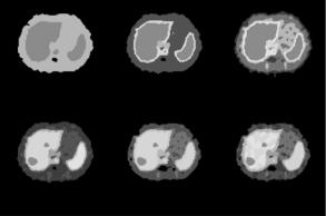
Figure 3.9 shows the segmentation results using different numbers of clusters, k, in the clustering algorithm. The number of clusters is actually varied from 3 to 13 but only some representative samples are shown. In each of the images in Figs. 3.9(a)–3.9(f), different gray levels are used to represent the cluster locations. Figure 3.9 shows that when the number of clusters is small, segmentation
150 |
Wong |
a |
b |
c |
d |
e |
f |
Figure 3.9: Tissue segmentation obtained with different number of clusters.
(a) k = 3, (b) k = 5, (c) k = 7, (d) k = 8, (e) k = 9, and (f) k = 13. (Color Slide)
of the data is poor. With k = 3, the liver, marrow, and spleen merge to form a cluster and the other regions merge to form a single cluster. With 5 ≤ k ≤ 7, the segmentation results improve because the blood vessels and stomach are visualized. However, the hepatic tumors are not seen and the liver and spleen are classified into the same cluster. With k = 8, the tumors are visualized and almost all of the regions are correctly identified (Fig. 3.9(d)). Increasing the value of k to 9 gives nearly the same segmentation as in the case of k = 8 (Fig. 3.9(e)). Further increasing the value of k, however, may result in poor segmentation because the actual number of tissues present in the data is less than the specified number of clusters. Homogeneous regions are therefore fragmented to satisfy the constraint on the number of clusters (Fig. 3.9(f)). Thus, 8 or 9 clusters appear to provide reasonable segmentation of tissues in the slice and this number agrees with the various kinetics present in the data.
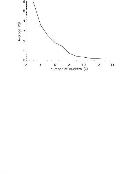
Figure 3.10 plots the average MSE across clusters as a function of k. The average MSE decreases monotonically, as it drops rapidly (k < 8) before reaching a plateau (k ≥ 10). From the trend of the plot, there is no significant reduction in the average MSE with k > 12. Furthermore, the decrease in the average MSE is nearly saturated with k ≥ 8. These results confirm the findings of the images in Fig. 3.9, suggesting 8 or 9 as the optimal number of clusters for this dataset.
Table 3.1 tabulates the results of applying AIC and SC to determine the optimum number of clusters which is the one that gives the minimum value for
Medical Image Segmentation |
151 |
|||||||||||||
|
|
|
|
|
|
|
|
|
|
|
|
|
|
|
|
|
|
|
|
|
|
|
|
|
|
|
|
|
|
|
|
|
|
|
|
|
|
|
|
|
|
|
|
|
|
|
|
|
|
|
|
|
|
|
|
|
|
|
|
|
|
|
|
|
|
|
|
|
|
|
|
|
|
|
|
|
|
|
|
|
|
|
|
|
|
|
|
|
|
|
|
|
|
|
|
|
|
|
|
|
|
|
|
|
Figure 3.10: Average mean squared error (MSE) as a function of number of clusters.
the criteria. Both criteria indicate that k = 8 is an optimal approximation to the underlying number of kinetics. It was found that a good segmentation can be achieved when the number of clusters is the same as that determined by the criteria. Conversely, the segmentation result is poor when the number of clusters is smaller than that suggested by the criteria and there is no significant improvement in segmentation when the number of clusters is larger than that determined by the criteria. The heuristic information given by both criteria also support our visual interpretation of the clustering results, suggesting that the criteria are reasonable approaches to objectively determine the number of clusters.
Table 3.1: Computed values for AIC and SC with different choices of the
value of k
|
|
|
|
|
Number of clusters, k |
|
|
|
|
||
|
|
|
|
|
|
|
|
|
|
|
|
Criterion |
3 |
4 |
5 |
6 |
7 |
8 |
9 |
10 |
11 |
12 |
13 |
|
|
|
|
|
|
|
|
|
|
|
|
AIC |
99005 |
95354 |
93469 |
90904 |
88851 |
86967a |
89769 |
93038 |
91994 |
90840 |
89807 |
SC |
98654 |
94888 |
92887 |
90206 |
88038 |
86038a |
88725 |
91878 |
90719 |
89450 |
88301 |
|
|
|
|
|
|
|
|
|
|
|
|
AIC: Akaike information criterion; SC: Schwarz criterion.
a Values in bold correspond to the computed minimum of the criterion.