Kluwer - Handbook of Biomedical Image Analysis Vol

5.4.2.1 Manual Measurements

Manual measurements of arterial diameter were performed in 117 frames corresponding to four sequences of different image quality. Three experts assessed each frame twice in independent sessions. In each sequence several frames were measured: 1 out of 10 in phase B1 (frame number 1, 11 . . . 61) and 1 out of 50 during the rest of the test (frame number 101, 151 . . . ). Depending on the duration of the sequence the total number of measured frames was between 28 and 30 per sequence.

Each diameter measurement was obtained by manually fitting a spline to the inner contour of each arterial wall. The diameter was defined as the average distance between both spline curves (see Appendix 5.8). The vasodilation measurements were obtained by dividing the manually obtained diameters by the average diameter over phase B1; the dilation was finally expressed as a percentage, getting %FMD values as defined before.

Gold-standard measurements were derived from these 117 frames. The grand-average of the six diameter measurements done by the three observers is considered the gold-standard arterial diameter estimate for each frame. The gold-standard dilation measurements are obtained by dividing these estimated diameters by the grand-average diameter over phase B1 for each sequence, to get %FMD values. Accuracy, reproducibility, and intraand interobserver variability of manual measurements were analyzed:

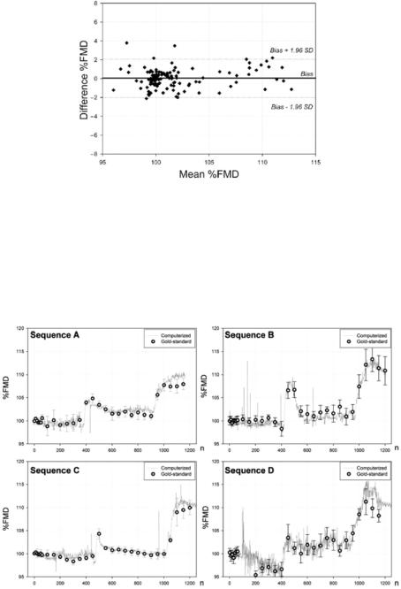
(i)Accuracy. Figure 5.7 shows the Bland–Altman plots comparing the intersession average measurement for each observer and the gold-standard measurements. The biases and standard deviation of the differences for

Figure 5.7: Bland–Altman plots comparing the intersession measurement average versus the gold-standard measurements. The horizontal and vertical axes indicate the average %FMD and the difference %FMD, respectively.

Bias and standard deviation of the differences (SDc ), corrected for repeated measurements, between manual and gold-standard %FMD measurements. SDa and SDw stand for the SD of the differences of the intersession average and the within-observer variability.

the three observers are given in Table 5.3. Standard deviations are corrected to take into account repeated measurements according to the method proposed by Bland and Altman [26].

(ii)Reproducibility. The CV of each group of six measurements is calculated for each one of the 117 manually measured frames. This CV is averaged for all the frames of each one of the four sequences, being considered the CV of the manual measurement for each sequence. These four values are averaged finally, obtaining an overall reproducibility value for manual measurements in our study. The results are shown in Table 5.4.

(iii)Interand intraobserver variability. Figure 5.8 shows Bland–Altman plots comparing both sessions of each observer. In order to estimate the overall interand intraobserver variability of manual measurements (with correction for repeated measurements) we carried out the procedure proposed by Bland and Altman in [27]. To this end, a two-way Analysis of Variance (ANOVA) with repeated measurements was performed

Table 5.4: Reproducibility of manual and automated measurements

Mean and SD of CV (%) measured with respect to %FMD value.

Figure 5.9: Bland–Altman plot comparing the automatic measurements (using normalized mutual information as similarity measure) versus the gold standard. The horizontal and vertical axes indicate the average %FMD and the difference %FMD of the automatic measurements and the gold-standard measurements, respectively.

Figure 5.10: FMD curves obtained by the proposed automated method (–) and by the gold-standard measurements (•). Error bars show the 95% confidence interval of the gold-standard measurements for comparison.

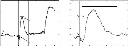
Figure 5.11: Definition of the segment of analysis for principal component analysis (PCA). (a) The original curve with indication of the instant of cuff release (first discontinuous vertical line), and start- (ncuff + 15 sec) and end-points (206 sec later) for PCA (second and third disconstinuous vertical lines); horizontal solid lines indicate the maximum flow-mediated dilation (FMD) and basal FMD levels used for the computation of classical FMDc. Horizontal solid lines indicate the maximum FMD ( max) and basal FMD levels ( basal), which are relative to a reference frame ( r). (b) A zoom into the segment that will undergo PCA. The segment of analysis is indicated with a thick solid line.

To be more specific, let CT (n) be an FMD curve (Fig. 5.11(a)). In order to analyze only FMD effects, a segment of this curve, C(n), was selected for PCA (Fig. 5.11(b)). This segment is defined to have a duration of D = 206 sec starting d = 15 sec after the release of the cuff pressure. In this way, all segments are synchronized with the FMD onset and have the same duration, which in our acquisition protocol is enough to reach the post-FMD basal level in all subjects without overlapping with the NMD test. We disregard the first 15 sec since that portion of the curve is mostly noisy due to motion artifacts. FMDc values were also measured by visually selecting the maximal and basal FMD levels. Since the whole curve is relative to the diameter of the reference frame, FMDc can be calculated directly from this plot. By considering the C(n) curve as a

D-dimensional vector, c, ROBPCA will be applied to the vector set {ci/Ci(no)}, of normalized relative values, where i = 1 . . . n is the subject index. In our experience, it is convenient to compute the EigenFMD modes with respect to a frame that represents the basal level, hence the division by Ci(no) (cf. next

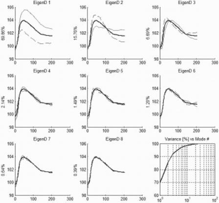
section). This renormalization corrects for small fluctuations in the baseline due to patient movements in the maneuver of cuff deflation, which themselves can introduce artifactual variation into the statistical analysis. This experiment contains n = 161 subjects, whose curves did not have any apparent artifacts in the FMD segment. Figure 5.12 shows the resulting eigenmodes of the relative FMD curves, which will be referred as EigenFMD modes in the sequel.

Figure 5.12: Representation of the variation explained by the first eight eigenFMD modes. The average flow-mediated dilation (FMD) curve, and the curves resulting of adding/subtracting the corresponding EigenFMD mode of variation to the mean, weighted by one standard deviation, are plotted in bold line and in thin solid/dashed lines, respectively. The y-axis label of each EigenFMD plot indicates the percentage of variance explained by the corresponding EigenFMD. The lower-right plot shows the accumulated percentage of variance versus the number of EigenFMD modes taken into account. EigenFMD modes were computed using the ROBPCA method.

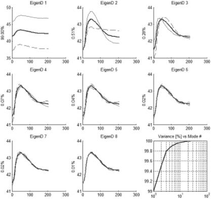
A similar analysis can be performed by applying the ROBPCA technique to the curves of absolute diameter. This analysis can now reveal correlations between risk factors and the absolute vessel diameter as evidenced by some previous clinical studies. To this end, we manually measured the diameter of the reference frame of each subject, r, using the technique presented in Appendix 5.8. Subsequently, each vector ci was unrelativized according to cia = ci · r. Figure 5.13 shows the corresponding modes, which are referred as EigenD

Figure 5.13: Representation of the variation explained by the first eight EigenD modes. The average diameter curve, and the curves resulting of adding/subtracting the corresponding EigenD mode of variation to the mean, weighted by one standard deviation, are plotted in bold line and in thin solid/dashed lines, respectively. The y-axis label of each EigenD plot indicates the percentage of variance explained by the corresponding eigenmode. The lower-right plot shows the accumulated percentage of variance versus the number of EigenD modes taken into account. EigenD modes were computed using the ROBPCA method [33].