

Kluwer - Handbook of Biomedical Image Analysis Vol
.2.pdf282 |
Yang and Mitra |
 (a) T11mm30_90.raw
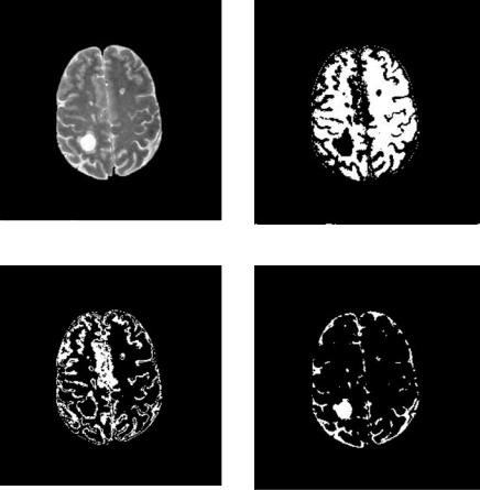
(b) CSF gray-level truth model (c) Gray matter gray-level truth model
(d) White matter gray-level truth model
Figure 6.5: Noisy MRI and the corresponding truth model for CSF, gray matter, and white matter.
The truth models are originally fuzzy models (Figs. 6.5(b)–6.5(d)). Since all results produced from the algorithms are hard clustering, the fuzzy truth models are converted into hard models by classifying a pixel to the category in which it has the largest pixel value.
Misclassification results (in Figs. 6.6–6.9) show that DA and AFLC perform better than k-means and FCM, demonstrating the effectiveness of the advanced algorithms in being more noisy tolerant.
6.4.1.2 Segmentation of Lesions in Multiple Sclerosis from MRI
Segmentation of MS lesions from simulated MRI: It is difficult to partition MS from T1-, T2-, or PD-weighted images because of the lack of intensity difference between MS lesion and other brain tissues, as is illustrated in Figs. 6.10(a)– 6.10(c). It can be expected that when a pattern recognition technique

(a) Classified CSF |
(b) Classified gray matter |
(c) Classified white matter |
(d) Misclassification: 9.01% |
(e) Misclassification: 10.27% |
(f ) Misclassification: 5.29% |
Figure 6.6: Segmentation of noisy MR image by AFLC.
(a) Classified CSF |
(b) Classified gray matter |
(c) Classified white matter |
(d) Misclassification: 10.48% (e) Misclassification: 10.47% (f) Misclassification: 5.10%
Figure 6.7: Segmentation of noisy MR image by DA.
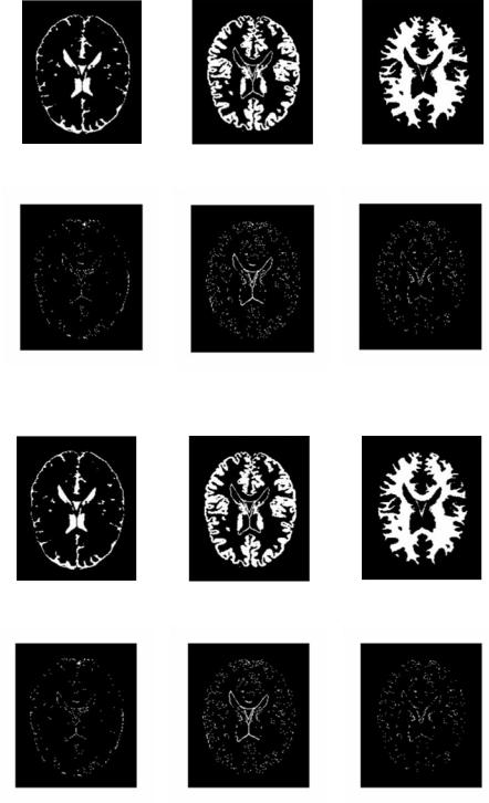
(a) Classified CSF |
(b) Classified gray matter |
(c) Classified white matter |
(d) Misclassification: 12.47% |
(e) Misclassification: 12.08% |
(f) Misclassification: 5.12% |
Figure 6.8: Segmentation of noisy MR image by k-means.
(a) Classified CSF |
(b) Classified gray matter |
(c) Classified white matter |
(d) Misclassification: 12.36% |
(e) Misclassification: 12.04% (f) Misclassification: 5.12% |
Figure 6.9: Segmentation of noisy MR image by FCM.

Statistical and Adaptive Approaches for Optimal Segmentation |
285 |
(a) T1-weighted MRI |
(b) T2-weighted MRI |
(c) PD-weighted MRI |
(d) T1-weighted MRI without |
(e) T2-weighted MRI without |
(f) PD-weighted MRI |
extraneous parts |
extraneous parts |
without extraneous parts |
(g) Synthesized image (T1- |
(h) Fuzzy MS lesion truth |
(PD-T2)) |
model |
(i) Hard MS lesion truth model
(j) k-means-segmented MS |
(k) AFLC-segmented MS |
(l) DA-segmented MS |
lesion |
lesion |
lesion |
Figure 6.10: Segmentation of MS lesions.
286 |
Yang and Mitra |
is applied, the lesions will be classified either with gray matter in Figs. 6.10(a) and 6.10(c) or CSF in Fig. 6.10(b) since the intensities of the lesions are similar to those tissues. It is a common practice that information embedded in multichannel MR images are combined to extract MS lesions [35, 36]. In this example, a synthesized image is created by manipulation of the three images: synthesized image = T1 − (PD − T2). Figure 6.10(g) shows the synthesized image of slice #90 T1-, T2-, and PD MR images, respectively. It can be seen that Fig. 6.10(g) provides distinct intensity level variation among gray matter, white matter CSF, and MS lesions. Then synthesized image is feed into four clustering algorithms. Segmentation results are shown in Figs. 6.10(j)–6.10(l). Figure 6.10(h) is the fuzzy MS lesion truth model. A hard model in Fig. 6.10(i) is created by verifying that the fuzzy model possesses the largest value among other tissues at the same pixel. It can be observed that DA provides the closest result to the truth model.
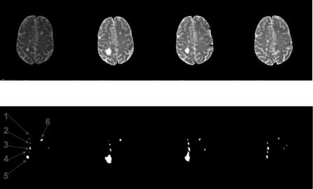
Segmentation of MS lesions from clinical MRI: Clinical MRI is much more complicated than simulated MRI in noise, clarity, and intensity inhomogeneity. The MR images to be segmented in the following example come from clinical data. The T2-weighted MR images are obtained from [33]. Four images are extracted from a MPEG movie showing chronic progression of MS lesions (Figs. 6.11(a)–6.11(d)). The images have been compressed, showing poor image
(a) |
(b) |
(c) |
(d) |
(e) |
(f ) |
(g) |
(h) |
Figure 6.11: MR images with MS lesions in chronic order, segmentation and
labeling.
Statistical and Adaptive Approaches for Optimal Segmentation |
287 |
resolution and reduced quality (with observable blocking artifacts.) The results of segmentations on these images are summarized in Figs. 6.11(e)–6.11(h), with labeling of the individual lesions shown in Fig. 6.11(e). Segmentation processes will be explained below. With image (a) and (b), intermediate results are shown in Figs. 6.12 and 6.13. For image (c) and (d), intermediate results are skipped and only the white matter masks and final segmentations are illustrated in Figs. 6.14 and 6.15.
Segmenting MS lesions from a single modality image such as the one used in this example is difficult as has been explained in the previous section. However, when images in other modalities are not available, background knowledge can be used. As most of the MS lesions occur in the white matter, Johnston et al.
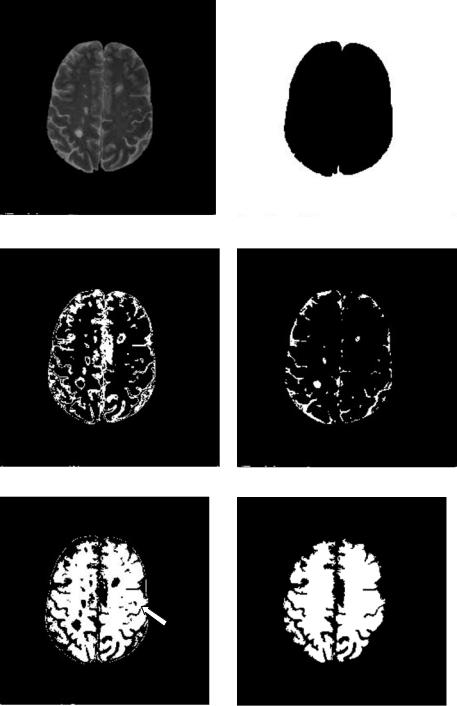
[35] suggested creating a white mask to confine segmentation area such that segmentation accuracy can be enhanced. In this case, segmentation is a twopass process. The image is first roughly segmented into four categories with DA: the background, the white matter, gray matter, and CSF and other tissues (Figs. 6.12(b)–6.12(e)). Not surprisingly, the MS lesions cannot form a class of their own. They are classified either as gray matter or other categories. Then a white matter mask is generated by morphological filtering of the white matter. This is shown in Fig. 6.12(f). Using this mask, a tailored image containing only the masked area is obtained (Fig. 6.12(g)) and used as input image in the second pass DA clustering. Final segmentation for Fig. 6.12(g) is shown in Fig. 6.12(h). The result is superposed on the original image in Fig. 6.12(i).
Besides being affected by the image quality, the above segmentation is influenced by the mask. The misclassification of gray matter into MS lesion on the right-hand side of the image (indicated by the red arrow in Fig. 6.12) in this example is caused by misclassification of gray matter into the white matter mask.
One of the goals to segment the lesions is to provide quantitative analysis. Once the lesions are segmented and labeled, progress of each lesion in size can be obtained in chronic order. Table 6.1 summarizes the changes in size (number of pixels) of all lesions that exist through all four MR images.
6.4.2Retinal Image Segmentation from Stereo Fundus Images
Objects such as blood vessels, optic disk, and optic cup in retinal images are crucial in monitoring and detecting the progression of retinal diseases such as vascular diseases, glaucoma hypertension, and diabetic retinopathy.
288 |
Yang and Mitra |
(a) Original image |
(b) First pass segmentation: background |
(c) First pass segmentation: CSF and other |
(d) First pass segmentation: gray matter |
(e) First pass segmentation: white matter |
(f ) White matter mask |
Figure 6.12: DA segmentation of MS lesions from Fig. 6.11(a).
Statistical and Adaptive Approaches for Optimal Segmentation |
289 |
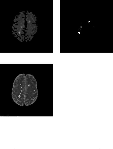
(g) Input image for second pass clustering |
(h) MS lesion segmented from the second |
|
pass |
(i) Segmented lesion overlay on (a)
Figure 6.12: (cont.)
Table 6.1: Segmented lesion size in chronic MR images
MR image |
L1 |
L2 |
L3 |
L4 |
L5 |
L6 |
|
|
|
|
|
|
|
(a) |
4 |
4 |
28 |
2 |
70 |
36 |
(b) |
2 |
15 |
29 |
1 |
401 |
32 |
(c) |
10 |
31 |
63 |
313a |
|
24 |
(d) |
0 |
11 |
45 |
14 |
41 |
16 |
|
|
|
|
|
|
|
a Lesions 4 and 5 merge in (c).
290 |
Yang and Mitra |
(a) Original image |
(b) First pass segmentation: white matter |
(c) First pass segmentation: CSF and other |
(d) First pass segmentation: gray matter |
Figure 6.13: DA segmentation of MS lesions from Fig. 6.11(b).
Segmentation of the extracted features allows us to investigate the effect of occlusion induced by these features in generating stereo disparity mapping and 3-D visualization of the optic cup/disk, leading to more accurate diagnosis or monitoring of glaucoma. This is a challenging task due to poor and nonuniform illumination of most fundus images and lack of standardized parameters for stereo imaging geometry.
6.4.2.1 3-D Segmentation of the Optic Disk/Cup
The onset and progression of glaucoma can usually be found or monitored through the measurement of changes in the optic disk and optic cup area. It

Statistical and Adaptive Approaches for Optimal Segmentation |
291 |
(e) White matter mask |
(f ) Input image for second pass segmentation |
(g) Segmented MS lesions |
(h) Segmented lesion overlay on (a) |
Figure 6.13: (cont.)
can be expressed as the cup-to-disk ratio in diameter (2D) or volume (3D), for which segmentation of the optic cup/disk in 2D or 3D is necessary. The cup-to- disk ratios obtained from 3-D visualization of the optic cup/disk has been found to match closely with those provided by physicians [48]. Semiautomated methods for finding the contours of the optical nerve head (ONH) by digital image analysis attempt to find the disparities of pixels between the fundus stereo pairs in a region including the ONH. Recent studies [48–50] describe in detail the algorithms developed for feature extraction, registration, correlation, and dynamic programming leading to computing disparities based on a nonconvergent stereo