

Kluwer - Handbook of Biomedical Image Analysis Vol
.2.pdf292 |
Yang and Mitra |
(a) Original image |
(b) White matter mask |
(c) Segmented lesion overlay on (a) |
(d) Segmented lesions |
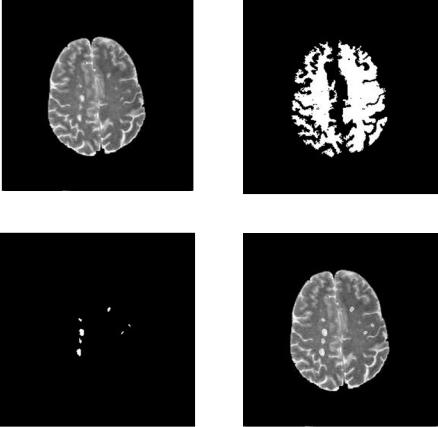
Figure 6.14: DA segmentation of MS lesions from Fig. 6.11(c).
imaging system. However, fully automated methods of finding precise disparities between a pair of stereoscopic images may still be problematic due to the presence of noise, occlusions, distortions, and lack of knowledge of the stereo imaging parameters. Under certain constraints, 3-D surface recovery of the optic cup/disk is possible from a pyramidal surface-matching algorithm based on the recovery of the optimum surface within a 3-D cross-correlation coefficient volume via a two-stage dynamic programming technique. The accuracy of the disparity map algorithm leading to 3-D surface recovery is highly dependent on the initial feature extraction process and the stereo imaging parameters.
The stereo images of a real world scene are taken from two different perspectives. The coordinate associated with depth of this scene can be extracted by triangulation of corresponding points in the stereoscopic images [51, 52]
Statistical and Adaptive Approaches for Optimal Segmentation |
293 |
(a) Original image |
(b) White matter mask |
(c) Segmented lesion overlay on (a) |
(d) Segmented lesions |
Figure 6.15: DA segmentation of MS lesions from Fig. 6.11(d).
assuming a nonconvergent imaging system. However, the geometrical information of the viewing angles when fundus images are taken in a clinical set-up are not documented, thus introducing certain ambiguities in the disparity mapping of the corresponding points in the stereo pairs. The overall process for 3-D visualization of retinal structures from stereo image pairs is complex and includes different matching strategies, area or feature based or a combination of both. Several preprocessing steps are also followed for feature extraction and registration prior to coarse to fine disparity search.
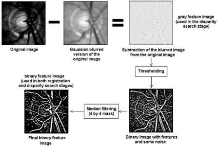
In the preprocessing stage, three channel (RGB) decomposition is first performed on the original color pair. Only the green channel is processed since it is the one that carries the most information. Red and blue channels have low

294 |
Yang and Mitra |
entropy in relation to the green channel and therefore are not taken into account. The registration process removes all vertical displacements leaving only the horizontal shifts arising from the different positions of the camera while taking the stereo fundus images. A good registration is crucial to obtain accurate disparity maps. A power cepstrum-based registration that uses Fourier spectrum properties to correct rotational errors that may be present in the stereo pair is employed. This process begins by extracting the most relevant features such as the blood vessels in both images. These features are extracted by subtracting a filtered version of the original stereo pair from the original (unsharp masking). After binarizing this new stereo pair, multiple passes of a median filter are used to eliminate some of the resulting noise in the images. Compensation for rotational differences is also performed via zero mean normalized crosscorrelation(ZNCC) [53] of the Fourier spectrum of the images using ZNCC as a disparity measure. ZNCC is expressed as follows:
covi, j ( f, g)
C(i, j) = (6.19)
σi, j ( f ) × σi, j (g)
1 |
i+K |
|
j+L |
|
|
|
|
|
|
|
|
covi, j ( f, g) = |
|
|
|
|
|
|
|
||||
|
|
|
|
|
fm,n − fi, j |
|
gm,n − |
|
|
||
|
m i |
|
|
|
|
gi, j |
|||||
((2K + 1)(2L + 1) − 1) |
K n |
j |
L |
|
|||||||
|
|
= − |
= − |
|
|
|
|
|
|
|
|
(6.20)
where f and g are the windows of pixels to be measured and f and g are corresponding average values. K and L define the size of those windows, and the indices for the pixels within the windows are i and j. σ ( f ) and σ (g) are the square roots of the covariances cov( f, f ) and cov(g, g), respectively.
According to the inherent Fourier spectrum properties, a rotation in the spatial image results in the same amount of rotation of its spectrum. Thus it is possible to find the angle of rotation of one image in the stereo pair with respect to the other by performing step-by-step rotations and cross correlating their Fourier transforms. The actual angle of rotation will be the one with the highest cross-correlation obtained. Rotational compensation is applied once the angle of rotation has been found.
After the rotational correction, a cepstrum transformation is applied to the sum of the binary-featured stereo pair images. The power cepstrum P is defined as in [52]:
P [i(x, y)] = |F(ln{|F[i(x, y)]|2})|2 |
(6.21) |
Statistical and Adaptive Approaches for Optimal Segmentation |
295 |
where F represents the Fourier transform operation. Let w(x, y) be the reference image, w(x + x0, y + y0) be the shifted image, and i(x, y) = w(x, y) + w(x + x0, y + y0). Then the power cepstrum of the sum of both images is given as
P[i(x, y)] = P[w(x, y)] + Aδ(x, y)
+ Bδ(x ± x0, y ± y0) + Cδ(x ± 2x0, y ± 2y0) + · · · (6.22)
where δ(x, y) is the Kronecker delta and A, B, and C are the first three coefficients for this power cepstrum expansion series [54]. Equation (6.22) shows that the displacement between images results in the sum of the power cepstrum of the original image w(x, y) plus a multitude of delta functions. Each delta is separated from the others by an integer multiple of the actual displacement we are looking for. In order to enhance the cepstral peaks, the cepstrum of the reference must be subtracted from the cepstrum of the stereo pair. With this in mind, a fixed number of deltas are chosen from the resulting cepstrum. Each delta represents a translational shift, or an integer multiple of the shift, of a pixel in the image shifted from the corresponding pixel in the reference image. All points are tested by cross correlating the reference image with the other image shifted by the number of pixels (in the vertical and horizontal directions) indicated by the current point being tested. The highest correlation will correspond to the most probable relative translation between both images.
Before disparity mapping is carried out, salient features of the image, such as the blood vessels, have to be extracted. The blood vessels are segmented through series of traditional local operation, such as unsharp masking, thresholding, and median filtering. This process is illustrated in Fig. 6.16.
The algorithm developed for the search of disparities first divides both images into square windows of a given size (multiple of two), say N by N. ZNCC is performed between the windows in one image with the windows in the other image. If cross correlation is larger than a certain threshold, it is assumed that the windows at that position in the image are similar, so the cepstrum is applied to those windows to check for possible shifts. Otherwise, if the cross correlation is smaller than or equal to the threshold mentioned, zero disparity is assigned to every pixel in the window. Only a specified number of horizontal points shown in the cepstrum are taken into account for analysis. Let’s say that, for an N by N window, only N/4 horizontal points are chosen for analysis in the cepstral plane. This is because for an N by N window the maximum horizontal displacement that can be detected is N/2 (either to the right or to the left, making a full range
296 |
Yang and Mitra |
Figure 6.16: Blood vessel extraction for registration and disparity mapping.
of N pixels), so checking all N/2 points for right and left shifts will be very time consuming. Instead, only the most probable N/4 horizontal shifts found by the cepstrum will be tested using the cross correlation technique. One of the images of the stereo pair is considered as the reference image and the other is the test image. Then, for every point chosen (from the cepstrum), cross correlation is applied between the reference window (in the reference image) and the other window (in the test image) shifted by the number of pixels determined by the cepstral shift. Since the cepstrum can detect only the amount of the shifts but not their direction (the cepstrum is symmetric about the origin), each point should be tested for left and right shifts. So when checking N/4 cepstral points, actually
N/2 positions are analyzed. The highest value in the cross correlation will be the most probable shift that will be assigned to all elements in the window currently being tested for disparity. The number of cepstral points is not a fixed parameter and can be modified. This modification will affect the processing time and the accuracy of the disparity map. Once all disparities have been calculated with a window size of N by N pixels, the size of the window is reduced by a factor of two and the whole process is repeated until the windows reach a predetermined size. Each disparity map (calculated at a given resolution) is accumulated by adding it to the previous disparity map. At the end of the process, the final disparity map
Statistical and Adaptive Approaches for Optimal Segmentation |
297 |
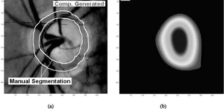
is the total accumulated disparity map. Usually the starting window size is 64 by 64 and the stopping size is 8 by 8. Smaller sizes of a window may not be worth computing because of the much longer time required and the small impact of it on the final disparity map. Also, since the window is so small, chances are that noise becomes a serious issue. The cepstrum is, in fact, a very noise tolerant technique that is suitable for finding disparities in chosen regions [55], while cross correlation is noise-sensitive and finds disparities using a procedure in a pixel-by-pixel fashion. A combination of both techniques results in an accurate and noise tolerant algorithm. In order to get an accurate 3-D representation from a stereo pair of images, disparities must be known for each point (pixel) of one image with respect to the other. Since the disparity search algorithm finds only disparities for the features or regions, disparities of all individual pixels are not known. The interpolation used here gives an estimate of the other missing disparities. Cubic B-spline is the interpolation technique applied to the sparse matrix resulting from the disparity search. It can be shown that the cubic B-spline can be modeled by three successive convolutions with a constant mask [54, 56]. In this case, a mask consisting of all ones of size 32 by 32 or 64 by 64 is used. After filtering the original sparse disparity matrix three times with the mask described above, a smooth representation results. This is the final 3-D surface of the ONH. With this surface, measures such as the disk and cup volume can be made. Figure 6.17(a) shows the optic disk/cup segmentation obtained from the
50 |
|
|
|
|
|
|
|
|
|
50 |
|
|
|
|
|
|
|
|
|
100 |
|
|
|
|
|
|
|
|
|
100 |
|
|
|
|
|
|
|
|
|
150 |
|
|
|
|
|
|
|
|
|
150 |
|
|
|
|
|
|
|
|
|
200 |
|
|
|
|
|
|
|
|
|
200 |
|
|
|
|
|
|
|
|
|
250 |
|
|
|
|
|
|
|
|
|
250 |
|
|
|
|
|
|
|
|
|
300 |
|
|
|
|
|
|
|
|
|
300 |
|
|
|
|
|
|
|
|
|
350 |
|
|
|
|
|
|
|
|
|
350 |
|
|
|
|
|
|
|
|
|
400 |
|
|
|
|
|
|
|
|
|
400 |
|
|
|
|
|
|
|
|
|
|
|
|
|
|
|
|
|
|
|
|
|
|
|
|
|
|
|
|
|
|
50 |
100 |
150 |
200 |
250 |
300 |
350 |
400 |
50 |
100 |
150 |
200 |
250 |
300 |
350 |
400 |
|||
|
|
|
|
|
|
|
|
|
|
|
|
|
|
|
|
|
|
|
|
|
|
|
|
(a) |
|
|
|
|
|
|
|
|
|
(b) |
|
|
|
|
|
Figure 6.17: Segmentation of optic disk/cup from 3-D disparity map. (color
slide)
298 |
Yang and Mitra |
above disparity mapping. The manual segmentation from an ophthalmologist is also shown for reference. Figure 6.17(b) is the smoothed disparity maps from which the iso-disparity contours were obtained.
6.4.2.2 Blood Vessel Segmentation via Clustering
Blood vessel segmentation has been a well-researched area in recent years, motivated by the needs such as image registration in our case, as well as in visualization and computer-aided surgery. A large number of vessel segmentation algorithms and techniques have been developed, oriented toward various medical image modalities, including X-ray angiography, MRI, computed tomography (CT), and other clinically used images. Like general image segmentation, vessel segmentation is also an application and image modality specific. It can be automatic or nonautomatic. According to a very thorough recent survey [57], vessel segmentation techniques can be roughly classified into the following categories (again, similar to general image segmentation, some techniques are integrated methods that combine approaches from different categories):
1.Pattern recognition techniques: This category includes multiscale approaches that extract large and fine vessels through low resolution and high resolution, respectively; skeleton-based approaches that extract blood vessel centerlines and connect them to form a vessel tree, which can be achieved through thresholding and morphological thinning; regiongrowing approaches that group nearby pixels that are sharing the same intensity characteristics assuming that adjacent pixels that have similar intensity values are likely to belong to the same objects; ridge-based approaches that map 2-D image into a 3-D surface, and then detect the ridges (local maximums) using various methods; differential geometrybased approaches; matching filter approaches; and morphological approaches.
2.Model-based methods: Model-based methods extract vessels by using explicit vessel models. Active contour (or snake) [58] finds vessel contours by using parametric curves that changes shapes when internal and external forces are applied. Level set theory [59] can also be adapted to vessel segmentation. Parametric models, template matching, and generalized cylinders model also fall into this category.
Statistical and Adaptive Approaches for Optimal Segmentation |
299 |
3.Tracking-based methods: Tracking-based approaches track a vessel from a starting point on a vessel, and detect vessel centerlines or boundaries by analyzing the pixels orthogonal to the tracking direction.
4.Artificial intelligence methods: These methods use the knowledge of targets to be segmented, for example, the properties of the image modality, the appearance of the blood vessels, anatomical knowledge, and other high-level knowledge as guidelines during the segmentation process. Low-level image processing techniques such as thresholding, simple morphological operations, and linking are employed depending on the guidelines.
5.Neural network-based methods: Neural networks are designed to learn the features of the vessels via training, in which a set of sample vessels containing various targeted features are fed into the network such that the network can be taught to recognize the object with these features. The capability of the trained network in recognizing vessels depends on how thorough the features are represented in the training set and how well the network is adjusted.
6.Tube-like object detection methods: This category represents other methods that extract tube-like objects and can be applied to vessel segmentation.
Some of the above approaches have been applied to retinal blood vessel segmentation. Chaudhuri et al. [60] used a tortuosity measurement technique and matching filter for blood vessel extraction and reported 91% of blood vessel segments and 95% of vessel network. Wood et al. [61] extracted blood vessels in the retinal image for registration by first equalizing the image with local averaging and subtraction, and then nonlinear morphological filtering was used to locate blood vessel segments. Hoover et al. [62] proposed an automated method to locate blood vessels in images of the ocular fundus. They used both local and global vessel features and studied the matched filter response using a probing technique. Zana and Klein [63] segmented vessels in retinal angiography images based on mathematical morphology and linear processing. FCM and trackingbased methods can also be used in retinal vessel segmentation [64]. Zhou et al.
[65] proposed an algorithm that relies on a matched filtering approach coupled with a priori knowledge about retinal vessel properties to automatically detect
300 |
Yang and Mitra |
the vessel boundaries, track the midline of the vessel, and extract useful parameters of clinical interest.
We can see from the previous section that accurate blood vessel segmentation is very important for registration and disparity mapping. The segmentation method described previously involves Gaussian filtering, unsharp masking, thresholding, and median filtering all of which can be easily affected by image illumination or contrast of the image. Here, we used advanced clustering approaches for the same task and compared it with the Gaussian filtering method.
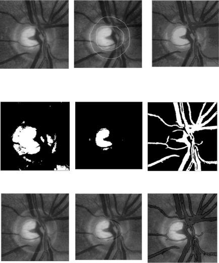
Among the three color channels, the green channel provides better contrast for edge information. Therefore, it alone can be used to accelerate subsequent segmentation processes. Challenge of blood vessel segmentation lies in distinguishing the blood vessel edges. However, most images are noisy and nonuniformly illuminated. In the optic disk area, blood vessel edges are smeared by reflectance. Simple segmentation techniques such as the one described above can produce noisy and inaccurate result. As is illustrated in Fig. 6.19(a), edges of the optic disk are mistakenly classified as blood vessel edges.
DA clustering solves this problem. Figure 6.18(c) shows the segmented result. Image resulted directly from DA segmentation is still affected by the noise in the original image, since single pixel intensity is used as feature. However, the noise in the segmented image can be easily removed through morphological filtering. The expansion or shrinking of blood vessel edges caused by morphological erosion and dilation can be corrected by edges detected by a simple edge detector, such as a Canny edge detector. Figure 6.18(d)–6.18(f) show the segmented optic disk, optic cup, and blood vessels in the ONH, respectively. The optic disk/cup segmentation is very similar to the manual segmentation in Fig. 6.18(b).
Blood vessels thus segmented are then used for registration and disparity mapping in the 3-D optic disk/cup segmentation, as is shown in Fig. 6.19(b). Three-dimensional visualization of the optic disk/cup with and without DA segmentation is comparatively demonstrated in Figs. 6.19(c) and 6.19(d). We can see that with DA segmentation, more accuracy is achieved.
6.4.3 Color Cervix Image Segmentation
Cervical cancer is the second most common cancer among women worldwide. In developing countries, cervical cancer is the leading cause of death from cancer. About 370,000 new cases of cervical cancer occur worldwide, resulting
Statistical and Adaptive Approaches for Optimal Segmentation |
301 |
(a) Fundus image (left stereo |
(b) Manually segmented optic (c) DA segmentation of (b) |
image) |
disk/cup by an ophthalmologist |
|
on the right stereo image |
(d) DA-segmented optic disk |
(e) DA-segmented optic cup |
(f) DA-segmented blood vessels |
(g) Final segmentation of optic |
(h) Final segmentation of |
(i) Final segmentation of blood |
disk |
optic cup |
vessels |
Figure 6.18: DA segmentation on clinical retinal image.
around 230,000 deaths each year. Cervical cancer develops slowly and has a detectable and treatable precursor condition known as dysplasia. It can be prevented through screening at-risk women and treating women with precancerous and cancerous lesions. In many western countries, cervical cancer screening programs have reduced cervical cancer incidence and mortality by as much as 90%. Analysis and interpretation of cervix images are important in early detection