

Kluwer - Handbook of Biomedical Image Analysis Vol
.2.pdf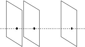
414 |
Xu et al. |
Ns,1
Ns,2
Ns,d
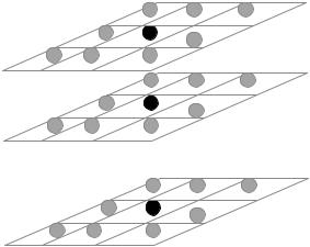
Figure 8.15: Illustration of a 3 by 3 by d neighborhood in mMRF model.
are the pixels in neighborhood. The prior probability of the whole image is
p(X) = Z exp − |
s |
Vs(x) = Z exp − |
s |
[VsN (s) + VsE (s)] . (8.43) |
||
1 |
|
|
1 |
|
|
|
Similar to the energy definition of monochrome image, the clique energy Vs(x) for mMRF model at location s is a summation of spatial constraint energy VsN (x) and edge constraint energy VsE (s) in all channels. Their definitions are given in the following equations, respectively:
d
VsN (s) = |
VsN,i(s), |
(8.44) |
|
i=1 |
|
|
d |
|
VsE(s) = |
|
|
VsE,i(s), |
(8.45) |
i=1
where the VsN,i(s) and VsE,i(s) represent the component in the ith dimension. Compared to the energy function in traditional mMRF models [46, 82, 83], an additional edge constraint VsE is added, which preserves the details of each dimension in the probability description and provides an even more accurate description of the energy function. This can makes the label updating process more sensitive at the regions boundaries.
Based on the above definition, we can find the a posteriori probability as
p(Y | X) p(Y | X) p(X) exp − |
s |
i 1 2ss2,i (ys,i − µs,i)2 |
|
||||||
|
|
|
|
|
d |
1 |
|
|
|
|
|
|
|
|
|
|
|
|
|
− |
|
|
|
|
= |
|
|
|
|
d |
(VsN,i(s) + VsE,i(s)) , |
|
|
(8.46) |
|||||
|
|
|
|
|
|
|
|
|
|
s i=1
416 |
Xu et al. |
with a Quad-Tree procedure, a “initial region merging” process is applied, in which a new region map is created as an initial segmentation result for the QHCF algorithm by combining all the regions found in different channels. The “merging” basically means the integration of region maps from all channels.
Under this presegmentation map, the definition of confidence for each pixel is the same as Eq. (8.29). However, the energy calculation is based on Eq. (8.47).
8.4.2.2.2 Dynamic Weighting. In multichannel data/image processing, different channels usually convey different amount of information. For example, in the soft tissue type identification with MR imaging [81], subjects are generally scanned with the multiple contrast weightings, such as T1-weighted (T1W), T2-weighted (T2W), proton density-weighted (PDW), and 3D time-of-flight (3D TOF). Since each contrast weighting imaging technique is sensitive only to certain tissue types, therefore, they usually contribute differently to the final decision when different tissue type is analyzed.
However, since there is no prior knowledge about the tissue type sensitivity layout in each channel, it is very impractical for human interaction involved in the segmentation process. In this study, a dynamic weighting system is proposed as a simulation of human’s decision process, which automatically decides the weighting coefficient for the energy calculation among channels. In our implementation, two factors are significant in managing the dynamic weighting:
1.Complexity factor (CF): It measures the amount of details that each channel provides at a certain location. In the surrounding region of each location, we assume the complexity is proportional to the number of edges. The more edge points can be detected, the more details this channel can provide. Since Canny Edge detector [15] has been used successfully in the energy calculation, it is utilized in our implementation to generate edge map. Based on the requirements of segmentation performance, two ways are proposed to evaluate the complexity factor.
(i)Local CF: The number of edge points within a local neighboring region in each channel.

Segmentation Issues in Carotid Artery Atherosclerotic Plaque |
417 |
(ii)Global CF: The number of edge points in the whole image in each channel (it is equivalent to local CF with neighboring range as the whole image).
Obviously, global CF is simple in terms of computation and represents the importance of each channel in a general sense. It is very efficient when one of channels plays a critical role in the segmentation process. On the other hand local CF is more complicated because it estimates the complexity of each channel at every location. However, it is very effective in preserving the segmentation details from each channel. Local CF is also very suitable to the situation where no prior knowledge of each channel’s potential contribution to segmentation results.
2.Weighting factor (WF): It is used to calculate the exact weighting of each channel based on the measurement of complexity factor. Assume the complexity factor from each channel is represented as: CFi, i = 1, 2, . . . , d, the weighting factor is denoted as
CFi
WFi = d , (8.50)
i=1 CFi
and the clique energy at each locataion Vs(x) in Eq. (8.9) can be computed
as
d
Vs(x) = WFi[VsN,i(x) + VsE,i(x)]. |
(8.51) |
i=1 |
|
8.4.2.3 Experiments and Discussion
Multiple contrast weighting MRI is an important imaging technique in clinical diagnosis. In this experiment, the mMRF version of QHCF algorithm (mQHCF) is applied on a set of ex-vivo atherosclerotic images.
Carotid endarterectomy specimens were scanned using a custom designed surface coil on a 1.5T GE SIGNA scanner with the following contrast weightings: T1W, T2W, PDW, and TOF. Based on observation and empirical knowledge, the tissues identified by T2W and PDW MR images are quite similar. To reduce computation complexity in the segmentation process, T2W images were removed, reducing the data space dimensions to three.
Figures 8.17(a)–8.17(c) show the original image scanned with T1W, T2W, and PDW, respectively. The circular shape object in the center of the image
418 |
Xu et al. |
|
|
|
|
|
(a) |
|
(b) |
|
(c) |
|
|
|
|
|
(d) |
|
|
|
|
|
|
(e) |
(f ) |
|||
|
(g) |
|
(h) |
|
(i) |
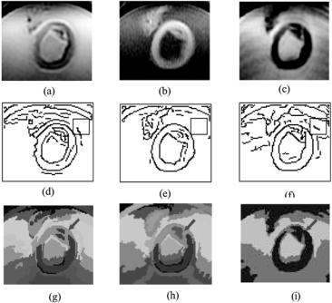
Figure 8.17: An example of ex-vivo atherosclerotic plaque segmentation with MCW MR images. (a)–(c) The region of interest in the original images in contrast weighing T1W, T2W, and PDW, respectively. (d)–(f) The corresponding edge maps by Canny edge detector. The square is an example of the region for local CF computing. (g) (color) Segmentation result by the proposed mMRF method with dynamic weighting. (h) (color) Segmentation result without dynamic weighting.
(i) (color) The segmentations with QHCF on PDW MR images only. The red arrows point the regions showing the different revilements of details with MCW w/n dynamic weighting and SWC segmentation methods.
is an intersection of carotid artery. Figures 8.17(d)–8.17(f) are the Canny edge maps. In this experiment, we use local complexity factor to control the channel weighting; the small square represents the size of local range for complexity calculation in each channel. Figure 8.17(g) shows the segmented result. Compared with the segmented results shown in Fig. 8.17(h) (applying mQHCF only without dynamic weighting) and Fig. 8.17(i) (applying QHCF only on PDW channel) we can observe the fact that (i) segmentation result with MCW reveals more details than that with SCW; (ii) MCW with dynamic weighting can reveals more details (as shown in the area those red arrows pointing).

Segmentation Issues in Carotid Artery Atherosclerotic Plaque |
419 |
|||||
Table 8.3: Workstation configuration |
|
|
||||
|
|
|
|
|
|
|
|
Workstation |
CPU |
Speed |
Memory |
OS |
|
|
|
|
|
|
|
|
|
Dell Precision 410 |
Intel PIII |
600 MHz |
256 MB Windows NT 4.0 |
||
|
|
|
|
|
|
|
Another factor deciding the algorithm’s performance is the processing time. Even though QHCF/mQHCF are deterministic implementations of the random field with finite optimization time, the computation is still a big cost for practical interactive applications. In mMRF, with the dimension expansion in the random field model, the amount of computation increases dramatically. This augment comes from two parts: (i) the computation used to calculate energy function and confidence for each location; (ii) the updating of its neighboring pixels. For other components in the optimization process, such as the updating of heap structure and searching of highest confidence, there is no big change involved. Since it is hard to compare the computation complexity theoretically, some experiments have been designed to compare the segmentation time for single modality image and multiple modality images. The experimental environment is set up as shown
in Table 8.3.
The proposed algorithm was applied on 50 multiple contrast weighing MR images for each image size, the average time used for segmentation are given in Table 8.4. As a comparison, the average segmentation time for single modality image (T1W) is also listed. These experimental results indicate that the computation used for mMRF model is larger than that for single contrast weighting
images.
Even though the discussion in section 8.4.2 has shown a solution for multiple channel image segmentation, there are some limitations in the applicability of
the proposed mMRF based algorithms:
Table 8.4: Average segmentation time
|
Single contrast |
Multiple contrast |
Image size |
weighting image (sec) |
weighting image (sec) |
|
|
|
128 × 128 |
13.202 |
92.104 |
256 × 256 |
37.531 |
244.328 |
512 × 512 |
69.459 |
517.163 |
420 |
Xu et al. |
(i)Low processing speed: From the experimental results in Table 8.4, the time used for multiple contrast weighting MR images is much longer than that for single contrast weighting ones, which is intolerable for practical interactive MR image analysis systems.
(ii)Independency assumption: In mMRF model, it is assumed that the signals in all the channels are regarded as independent as expressed in Eq. (8.42). However, in anthrosclerotic plaque study, even though the dependences among different contrast weighting images are unclear, there is no guarantee of their independency. Therefore, there is a risk that this assumption might be violated when new contrast weighting data is introduced.
8.4.3Clustering-Based Method
Even though the mMRF may provide a robust solution to the segmentation problem of multiple spectral data, the intrinsic limitations of this model discussed in section 8.4.2.3 may hinder its further application. Therefore, there is a motivation to pursue a more relaxed and practical approach that can satisfy the following conditions:
(i)No presumption on the distribution function of the multiple dimension data.
(ii)Fast processing speed that is suitable for interactive applications.
In this section, a nonparametric clustering algorithm was developed to fulfill the above requirements and employed to process the multiple contrast weighting MRI images.
8.4.3.1 Introduction
Clustering is generally regarded as an effective technique for automatic data grouping based on a given similarity measurement. In the clustering process, discrete objects can be assigned to groups that have similar characteristics. The object can be single value, such as pixel’s intensity in gray level image, or a vector in multidimensional data space. Generally, the clustering approaches usually consist of the following two steps:
Segmentation Issues in Carotid Artery Atherosclerotic Plaque |
421 |
(i)Cluster distribution or center searching.
(ii)Classification of dataset.
In the first step, the cluster center or the expression of density function is usually estimated so that the distribution of dataset can be clearly described. The second step is mainly on the dispatch of elements from the dataset based on certain criteria such as biggest similarity, shortest distance, maximum likelihood (ML), and K-nearest neighbor, etc.
8.4.3.1.1 Definition of Problem. First, we establish a clear definition of the studied problem. Suppose the number of MR imaging contrast weightings involved in the study is D, and images, Id, d = 1, . . . , D, are obtained from the same location of a patient’s carotid artery. Assuming that there is no motion between these acquisitions and all the images have the same dimensions, K = R × C, where R and C are the number of rows and columns of image. The data for each location k, k = 1, . . . , K, can be expressed as vk = [v1k, . . . , vDk]T , vdk Id, d = 1, . . . , D. vdk is the intensity value at pixel location k in the contrast weighting image d. Based on this, a d-dimensional space with dataset V = {vk, k = 1, . . . , K } is created. Our goal is to construct a new segmentation image (same as the label matrix defined in HCF study), which contains uniform regions, some of which will be the plaque tissues of interest in the cross sectional image of the carotid artery.
8.4.3.1.2 Data Cluster Center Searching. Based on the above definition of MCW MR image segmentation problem, the two steps in the clustering approaches can be described more specifically as (i) to estimate the cluster centers of the data vectors in the d-dimensional space and (ii) to partition the K data vectors into clusters by mapping them to the “nearest” cluster center under certain rules so as to generate the composite segmentation image.
Cluster center searching in multidimensional space is also called the multivariate location problem, and numerous nonparametric methods have been proposed [85, 86]. Among them, the minimum volume ellipsoid (MVE) estimator by Rousseeuw [87] is one of the most well-known solutions. It is defined as the ellipsoid that satisfies the following two conditions: (i) covering at least h elements of dataset V in d-dimensional space; (ii) the minimum volume. Then the center of this ellipsoid is regarded as the multivariate location estimate, the