

Kluwer - Handbook of Biomedical Image Analysis Vol
.2.pdf332 |
Walter and Klein |
detection algorithms (e.g., optic disk, macula, hemorrhages). Over and above that, it delivers landmarks for image registration.
7.5.1.2 Properties
Vessels are elongated features, much longer than, thick, reddish, and darker than the background. They enter the retina by the optic disk and go all over the retina forming the vascular tree.2 With increasing distance from the optic disk, the vessels become thinner and their contrast decreases. Contrast and color of vessels vary considerably from one image to another. Even in the same image, there may be color differences, as color depends on the vessel type (artery or vein), its diameter (the amount of hemoglobin that is transported), and the illumination of the retinal region where the vessel is situated.
The width of the thickest vessels is almost constant for all images taken with the same angle and the same resolution; we can state that all vascular structures in fundus images are thinner than a parameter λ (which depends on resolution and angle of the image).
As we have seen in section 7.2, vessels appear best contrasted in the green channel fg of the color images; our algorithm for vessel detection is exclusively based on the use of this channel. The main difficulties we have to deal with are as follows:
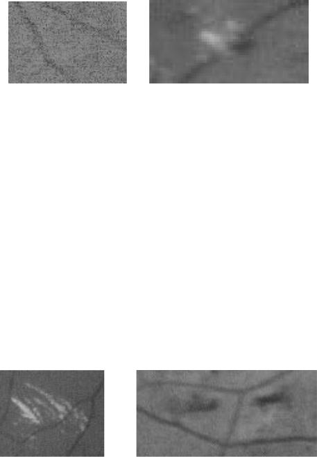
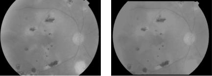
Often, retinal images are low contrasted and corrupted by noise. As a consequence, vessel contours are not well defined, and not all vessel pixels have a lower gray level than all the background pixels. However, the mean gray level on the vessel is lower than the mean gray level on the background (see also Fig. 7.12(a)).
The vascular tree may be interrupted by the presence of lesions (as shown in Fig. 7.12(b)) or noise.
The presence of exudates is a source of false detections, as the spaces between exudates have sometimes properties similar to vessels in terms of luminosity, width, and connectivity (see Fig. 7.13(a)).
2 The vascular tree as it appears in color images, is not a “tree” in the topological sense, as veins and arteries usually cross each other. It is more like a “net” of piecewise linear structures.
Analysis of Color Fundus Photos and Its Application to Diabetic Retinopathy |
333 |
(a) Two vessels corrupted by |
(b) A part of a vessel deconnected from the |
noise |
rest of the vascular tree by an exudate |
Figure 7.12: Main problems in vessel detection.
The presence of hemorrhages adds another source of false positives, as they have the same color. If they are connected to the vascular tree, they may be hard to distinguish from the vessels (see Fig. 7.13(b)).
7.5.1.3 State of the Art
There is a large variety of algorithms for vessel detection in retinal images. In most of these algorithms, vessels are modeled like piecewise linear segments with a Gaussian profile. Using linear or morphological filtering, features with this property are enhanced, other features are attenuated. This strategy has been proposed by Chaudhuri in [10] (linear filters) and by Zana in [11] (morphological filters). Drawbacks of these methods are the computational complexity due to directional filtering and some systematic errors on the borders of bright features (like the optic disk or hard exudates).
(a) Hard exudates close |
(b) Hemorrhages close to vessels |
to the vascular tree
Figure 7.13: Main reasons for false detections.

334 |
Walter and Klein |
Tracking algorithms are the second important group of vessel detection methods. These algorithms use the connectivity of the vascular tree as a main property. This is, in many images, not acceptable, particularly if lesions are present (see the Fig. 7.13(a)). Hence, this kind of approach must rely on good markers; then, tracking algorithms can, in our opinion, be powerful in detecting the vessel borders, but they are not adapted to detect the vascular structure.
7.5.1.4 The Algorithm
In this section, we present a new method for the detection of vessels in fundus images. The main idea is to detect thin structures in gray-scale images by evaluating the local contrast along watershed lines. This algorithm can also be applied to other problems where thin structures are to be found.
Prefiltering: As we can see in the Fig. 7.13(a), spaces between hard exudates are a systematic source of false positives for vessel detection algorithms. In order to remove small exudates, the prefiltered image p is calculated as follows:
p = γλa fg |
(7.13) |
with fg the green channel and γλa the area opening with the parameter λ. The result of this prefiltering step is shown in Fig. 7.14(b). One may notice that this filter is not very restrictive, the borders of the different features present in the image are not altered, but the small exudates are removed.
Extraction of dark details: Vessels appear as dark features in the green channel of a color image, their maximal width is known and does not vary with the image (as far as the resolution is the same). As we have seen in section 7.3,
(a) The green channel |
(b) The prefiltered image |
Figure 7.14: The prefiltering step: Small exudates are removed.
Analysis of Color Fundus Photos and Its Application to Diabetic Retinopathy |
335 |
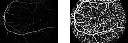
(a) The top-hat transformation of the |
(b) An approximation of the vascular |
prefiltered image |
tree |
Figure 7.15: Top-hat transformation and approximation of the vascular tree.
vessels can be removed from this image by means of the morphological closing with an appropriate size s1 (see also Fig. 7.6(c)). Calculating the difference to the original gives all the dark details that cannot contain the SE:
ϑ p = φs1 B( p) − p |
(7.14) |
In the top-hat image ϑ p (shown in Fig. 7.15(a)), vessels appear as bright features, elongated and connected. However, because of contrast differences between retinal images and between different vessels in one image, only a raw approximation of the vascular tree can be found by means of simple threshold techniques, as shown in Fig. 7.15(b). In our example, the vessels are obtained by an area threshold TK , proposed in [12]: The threshold is chosen in such a way that the resulting binary image contains at least K pixels.
Extraction of the crest lines: Considering the image shown in Fig. 7.15(a) as a topographic surface, we can notice that the vessels correspond to the crest lines in this image. An excellent tool for finding the crest lines in a gray-scale image has been presented in section 7.3: the watershed transformation. The strategy is to first find a good marker, then calculate the watershed transformation, and in the final step apply a contrast criterion in order to distinguish real vessels from false detection.
The usual technique to obtain a good segmentation result using the watershed transformation is to use markers (see section 7.3), i.e., the image is flooded only from “important” minima, the others are filled by means of the morphological reconstruction. Here, the markers must be chosen in such a way that the watershed line coincides with the vessels. It is, therefore, very important that
336 |
Walter and Klein |
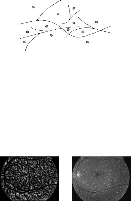
Figure 7.16: An ideal marker image (gray circles).
we mark all the “valleys” that are completely or partially surrounded by the crest lines. Such a marker is shown in the Fig. 7.16.
In order to obtain such a marker, we determine the points having maximal distance from the approximation shown in Fig. 7.15(b). In a first step, we fill the small “holes” of the thresholded image by a surface closing of small size, i.e., we remove all “holes” having less than 5 pixels, and then we invert the result and we determine the local maxima of the distance function:
m(x) = |
2 |
f (x) |
3if x ax {D(m1)} |
(7.15) |
|
m1 |
|
φλa TK |
( p) |
c |
|
= |
tmax |
|
if not M |
|
|
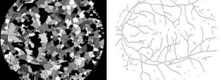
The distance function is shown in Fig. 7.17(a), its maxima superposed to the original image in Fig. 7.17(b). Of course, the presence of dark noise and features
(a) The distance image of the inverted |
(b) The marker image (here super- |
approximation |
posed to the green channel of the orig- |
|
inal image) |
Figure 7.17: A marker for vessel detection.
Analysis of Color Fundus Photos and Its Application to Diabetic Retinopathy |
337 |
(a) The watershed line and the catch- |
(b) The application of the contrast |
ment basins |
criterion |
Figure 7.18: The watershed line and the result of the application of the contrast criterion.
in the original image may produce a lot of spurious objects in the approximation image. As a consequence, there are more markers than necessary, but the number of minima has been significantly reduced, and the watershed line can now be determined:
WS |
m |
= |
f |
(7.16) |
( f ) |
|
WS(R (m)) |
Evaluation of the local contrast: The result of the watershed transformation is shown in Fig. 7.18(a). We note that on the one hand nearly all vessels coincide with a branch of the watershed line (WSL), but on the other hand, not all the branches correspond to vessels. Indeed, the high number of false positives (i.e., parts of the WSL that do not correspond to vessels) is a consequence of the fact that the WSL delimits the catchment basins. Hence, if a region is not completely enclosed by vessels, there is necessarily a branch of the WSL that does not correspond to a vessels. The nonideal marker adds even more false positives, for we do not have exactly one marker per entirely or partially enclosed region.
In order to remove these false positives, we have to analyze the WSL. We distinguish
bifurcation points (BIF): all points of the WSL that have more than two neighbors.
branches: all connected components of WSL\BIF(WSL). We call Fi, j the branch being the frontier between the two catchment basins CBi and CB j .
338 |
Walter and Klein |
Fi,j
Bj
Bi
Figure 7.19: Two catchment basins BVi and BVj and the frontier Fi, j between
them.
In the top-hat image, vessels appear brighter than the background (brighter than the adjacent regions) and changes in gray-level on the vessels are slow. Let us now consider two catchment basins CBi and CB j and the frontier Fi, j between them (see also Fig. 7.19). If Fi, j corresponds to a vessel, the mean gray-level value of the top-hat image on Fi, j must by higher than the mean gray level on the two catchment basins. Let ϑ p be the top-hat image and # A the number of pixels of the set A. We can then write the first criterion c1:
µFi, j = #{Fi, j } x Fi, j p2(x)
1
µBVi = #{BVi} x BVi p2(x)
c1(Fi, j ) = |
1 |
(µFi, j |
− µBVi ) + (µFi, j − µBVj ) |
(7.17) |
2 |
Evaluating the contrast criterion c1, all the false branches not coinciding with a dark detail extracted by the top-hat are removed. However, the result is not yet satisfying, because there are still false positives that are due to some small, not connected dark details like hemorrhages close to vessels producing also a quite high value for c1. In order to remove these false positives from the segmentation result, we have to take into consideration the local gray-level variation on the branch:
σFi, j = |
1 |
x Fi, j ( p2(x) − µFi, j )2 |
|
#{Fi, j } − 1 |
|
||
|
|
|
|
|
|
|
|
c2(Fi, j ) = c1(Fi, j ) − α · σFi, j |
(7.18) |
||
with α a weighting coefficient. With this enhanced contrast criterion, it is quite

Analysis of Color Fundus Photos and Its Application to Diabetic Retinopathy |
339 |
|
simple to distinguish between vessels and false positives: |
|
|
V1 = "i, j |
Fi, j with c2(Fi, j ) > β |
(7.19) |
The result V1 is shown in Fig. 7.18(b). We see that there are still small false positives. In fact, they are so small that the criterion c2 has no meaning. Therefore, we remove all the connected components of V1 that contain less than λ pixels (we chose λ = 30):
V = γλa(V1) |
(7.20) |
With this technique, we obtain very satisfying results, if the images do not contain larger exudates that have not been removed by the prefiltering step. Indeed, the spaces between exudates form small channels that are quite similar to vessels. One possibility is to calculate the mean gray level for the branches in the shade corrected image SCnorm and to use it as a complementary information: Only if the mean gray level is lower than a certain threshold, the branch is accepted. In this way, many false positives dues to exudates can be removed.
7.5.1.5 Results
The algorithm has been tested on sixty 640 × 480 fundus photographs taken with a Sony color video 3CCD camera on a Topcon TRC 50 IA retinograph. These images have not been used for the development of the algorithm. We asked an ophthalmologist to mark false detections and missed vessels on the result (a posteriori evaluation). We obtained a sensitivity of 83% and a predictive value of 97% an example is shown in Fig. 7.20.
(a) Original image (containing exu- |
(b) Segmentation result |
dates)
Figure 7.20: A result of the vessel detection algorithm.
340 |
Walter and Klein |
This kind of evaluation is certainly not the best method, as the expert is influenced by the result of the algorithm. However, vessels are clearly visible and an expert will always be able to mark them; the same holds for false positives. Over and about that, if an expert marks all vessels, it is far from being sure that he will not miss some of them, because this is a boring and time-consuming task.
7.5.2 The Detection of the Optic Disk
7.5.2.1 Motivation
The optic disk (or papilla) is one of the main features of the retina, its detection is essential for a system of automatic analysis of retinal images; it is the prerequisite for other segmentation algorithms (exudates, macula).
In the context of diagnosis of the glaucoma, the detection of and measures on the optic disk may also be of great importance. Hence, an algorithm of automatic detection of the optic disk is required.
7.5.2.2 Properties
The optic disk is the entrance of the optic nerve and the vessels into the retina. It is situated on the nasal side of the macula and it does not contain any photoreceptor: It is also called the blind spot. In color fundus photographs, the optic disk appears as a big bright spot of circular or elliptical shape, interrupted by the outgoing vessels. Its size varies from patient to patient, but its diameter is always comprised between 40 and 60 pixels in 640 × 480 images. The optic disk is characterized by a strong contrast between outgoing vessels and the bright color of the optic disk itself.
Unfortunately, this description is not valuable for all images: Sometimes, the contours are not clearly visible, the color tends more to a pale white, and there may be other regions in the image which are as bright or even brighter than the optic disk (due to nonuniform illumination or the presence of exudates).
7.5.2.3 State of the Art
In [13], the authors localize the optic disk using the high contrast between the papilla and the outgoing vessels. This method fails if there are exudates in the image.
Analysis of Color Fundus Photos and Its Application to Diabetic Retinopathy |
341 |
In [14], the authors use an area threshold for localization of the papilla, the Hough transform for the detection of its contours. The Hough transform is also used by [15]. The main problems that have been stated are low contrast and the case where its shape does not correspond to a circle (for example, if the optic disk is situated on the border of the image).
In [16], the authors use a template matching approach for the localization of the optic disk. The problem with this approach is the size variability of the papilla between different images and the presence of large accumulations of exudates.
7.5.2.4 The Algorithm
The presented algorithm can be subdivided into two parts: the localization and the detection of the contours of the optic disk. First versions of this algorithm have been presented in [17, 18].
Localization: As the optic disk belongs to the brightest parts of the image, the idea to apply an area threshold in order to find at least a part of the optic disk may work well, if there do not exist large accumulations of exudates or other bright regions. The atrophy in Fig. 7.21(a), for example, corresponds to a yellow spot and its size and shape are comparable to the one of the optic disk. Before we can apply a threshold to the image, it is therefore necessary to remove these bright features. This can be done using the vascular tree we have already detected: As the optic disk is the entrance of the vessels into the retina,
(a) The luminance channel of a retinal |
(b) The morphological reconstruction |
image containing an atrophy |
using the vascular tree |
Figure 7.21: The elimination of bright features.