

Kluwer - Handbook of Biomedical Image Analysis Vol
.2.pdf472 |
|
Suri et al. |
|
Image Volume |
|
|
Build Observation Vector |
|
Initial Centroid |
Observation Vector |
|
|
Get Current Centroid |
K |
Copy New Centroid |
Current Centroid |
|
to Current Centroid |
|
|
|
|
|
|
Membership Function Computation |
|
|
Membership Function |
|
|
New Centroid Computation |
|
|
New Centroid |
|
|
Compute Error ? |
|
Save Membership Function, Classified Image and Stop |
||
|
Stop |
|
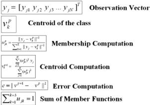
Figure 9.12: Fuzzy C mean (FCM) algorithm. Input is an image volume. An observation vector is built. Initially, the current centroid is given by the initial input centroid and K the number of classes. With the observation vector the membership function is computed, and with it a new centroid is computed. This new centroid is compared to the current centroid, and if the error is too large, the new centroid is copied into the current centroid and the process repeats. Otherwise, if the error is below the threshold, the membership function is saved, and the result is a classified image.
4.Convergence was checked by computing the error between the previous and current centroids ( v( p+1) − v( p) ). If the algorithm had converged, an exit would be required; otherwise, one would increment p and go to step 2 for computing the fuzzy membership function again. The output of the FCM algorithm was K sets of fuzzy membership functions. We were interested in the membership value at each pixel for each class. Thus, if there were K classes, then we threw out K number of images and K number of matrices for the membership functions to be used in computing the final speed terms.
Lumen Identification, Detection, and Quantification in MR Plaque Volumes |
473 |
Figure 9.13: Mathemetical expression of the FCM algorithm. Equations for the observation vector, centroid of the class, sum of the membership function, membership computation, centroid computation, and error computation are shown.
9.3.3 Graph-Based Segmentation Method
The graph segmentation method (GSM) segments an image by treating it as a graph G = (V , E) where V the set of vertices are the pixels and E the set of edges are pairs of pixels. Using a weight function w(e), where e is an edge (vi, v j ), the weights of the edges are computed and the edges are sorted by weight in a nondecreasing order. Initially, each pixel vi is segmented into its own component Ci.
For each edge (vi, v j ) in the list, a decision criterion D is applied and a decision is made whether or not to merge the components Ci and C j . After this decision is made on each edge in the list, the result is a list of the final components of the segmented image.
The input image is first smoothed by a given smoothing parameter σ . Input constant k determines the size preference of the components by changing the threshold function τ (C) (see Figs. 9.14 and 9.15).
The decision criteria D is a comparison between the difference between components Ci and C j and the minimum internal difference among Ci and C j . The difference between two components is defined as the minimum weight of the edges that connect the two components:
Dif Ci, C j ) = vi Ci,v j |
C j ,(vi,v j ) E w((vi, v j )). |
(9.12) |
|
( |
min |
|
|
|
|
|
|

 Smoothing parameter Smoothed Image; treat as graph
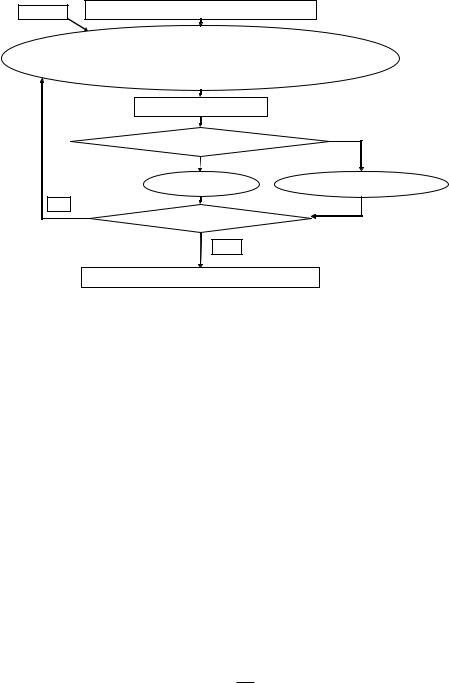
476 |
Suri et al. |
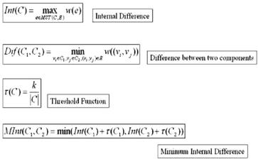
Figure 9.16: Graph segmentation method (GSM) equations. The internal difference of a component is the maximum edge weight of the edges in its minimum spanning tree. The difference between two components is the minimum edge weight of the edges formed by two pixels, one belonging to each component. The threshold function of a component is the constant k divided by the size of that component, where the size of a component is the number of pixels it contains. The minimum internal difference among two components is the minimum value of the sum of the internal difference and the value of the threshold function of each component.
If the difference between the two components is greater than the minimum internal difference among the two components, then the two components are not merged. Otherwise, the two components are merged into one component.
9.4Synthetic System Design and Its Processing
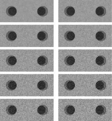
9.4.1 Image Generation Process
The model equation for generation of the observed image is shown in Eq. (9.16).
Iobserve = Ioriginal + η |
(9.16) |
Lumen Identification, Detection, and Quantification in MR Plaque Volumes |
479 |
|||||||||||||||||||||||
|
|
|
|
|
|
|
|
|
|
|
|
|
|
|
|
|
|
|
|
|
|
|
|
|
|
No. of Lumens |
|
|
|
|
|
|
Image Size: Rows and Columns |
|
|
|
|
|
|
Location of |
|
||||||||
|
|
|
|
|
|
|
|
|
|
|
|
|
|
|||||||||||
|
|
|
|
|
|
|
|
|
|
|
|
|
|
|
|
|
|
|
|
|
Lumens |
|
||
|
|
|
|
|
|
|
|
|
|
|
|
|
|
|
|
|
|
|
|
|
|
|||
|
|
|
|
|
|
|
|
|
|
|
|
|
|
|
|
|
|
|
|
|
|
|||
|
|
|
|
|
|
|
|
|
|
|
|
|
|
|
|
|
|
|
|
|
|
|
||
|
|
|
|
|
|
|
|
|
|
|
|
|
|
|
|
|
|
|
|
|||||
|
|
|
K |
|
|
|
|
Gray Scale Image Generation Process |
|
|
|
|
|
|
|
|
|
|||||||
|
|
|
|
|
|
|
|
|
|
|
|
|
|
|
|
|
|
|
|
|
|
|
|
|
|
|
|
Gaussian |
|
|
|
|
|
|
|
|
|
|
|
|
Mean, Var |
|
|
||||||
|
|
|
|
|
|
|
|
|
|
|
|
|
|
|
||||||||||
|
|
|
|
|
|
|
|
|
|
|
|
|
|
|
|
|
||||||||
|
|
|
|
|
|
|
|
|
|
|
|
|
|
|
|
|
|
|
|
|
|
|
|
|
|
|
|
|
|
|
|
|
|
|
|
|
|
|
|
|
|
|
|
|
|
|
|
|
|
|
|
|
|
|
|
|
|
|
|
|
|
|
|
Gray scale image with multiple lumens |
|
|
|
|
|
|
|
|
|
|
|
|
|
|
|
|
|
|
|
|
|
|
|
|
|
|
|
|
|
|
|
|
|
|
|
|
|
|
|
|
|
|
|
|
|
|
|
|
|
|
|
|
|
|
||||||
|
|
|
|
|
|
Classifier |
|
|
|
Lumen Detection and |
|
|
Region to Boundary |
|
||||||||||
|
|
|
|
|
|
|
|
|
|
|
|
|
|
|
|
|
|
|
|
|
|
|
||
|
|
|
|
|
|
|
|
|
|
|
|
|
|
|
|
|
|
|
|
|
|
|
||
|
|
|
|
|
|
CCA |
|
|
|
|
Quantification System (LDS) |
|
|
|
|
|
Overlays |
|
|
|||||
|
|
|
|
|
|
|
|
|
|
|
|
|
|
|
|
|
|
|
|
|
||||
|
|
|
|
|
|
|
|
|
|
|
|
|
|
|
|
|
|
|
|
|
|
|
||
|
|
|
|
|
|
|
|
|
|
|
|
|
|
|
|
|
||||||||
|
|
|
|
|
Binarization |
|
|
|
|
|
|
Ruler |
|
|
|
|
||||||||
|
|
|
|
|
|
|
|
|
|
|
|
|
|
|
|
|
|
|
|
|
|
|
|
|
Lumen Boundary Error & Overlays
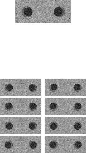
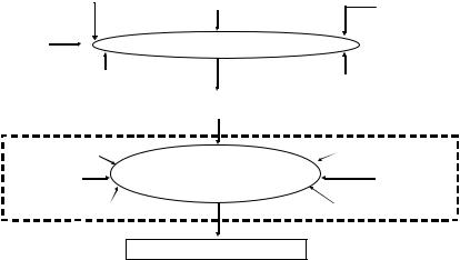
Figure 9.20: Block diagram of the system. A gray scale image is generated, with parameters being the number of lumens, location of lumens, the number of classes K , and a Gaussian perturbation with mean and variance. The result is an image with multiple lumens with noise. This image is then processed by the lumen detection and quantification system (LDS). This system includes many steps including classification, binarization, connected components analysis (CCA), boundary detection, overlaying, and measuring the error. The final result are the lumen errors and overlays.
generation process takes in the noise parameters: the mean and variance, the locations of the lumens, the number of lumens and the class intensities of the lumen core, the crescent moon, and the background.
Step two consists of lumen detection and quantification system (LDAS) (see Fig. 9.20). The major block is the classification system discussed in section 9.3. Then comes the binarization unit which is used to convert the classified input into the binarized image and also does the region merging. It also has a connected component analysis (CCA) system block which is the input to the LDAS. We also need the region-to-boundary estimator which will give the boundary of the left and right lumens. Finally we have the quantification system (called Ruler), which is used to measure the boundary error.
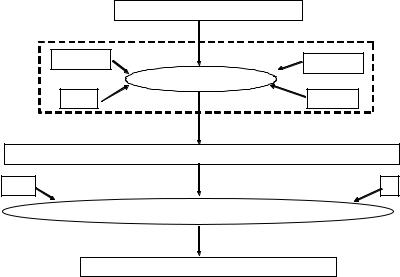
The LDQS system consists of lumen detection and lumen quantification system. The lumen detection system (LDS) is shown in Fig. 9.21. The detection process is done by the classification system, while the identification is done by the CCA system. There are three classification system we have used in our
Lumen Identification, Detection, and Quantification in MR Plaque Volumes |
481 |
Classified Image with Multiple Classes Inside Lumen
K (classes)
Detection: Class Merging &
Binarization
ROI
Lumen Regions Detected (2 Lumens here)
CCA
Left and Right Lumen Identification
Using CCA
Left Lumen & Right Lumens Identified
Figure 9.22: Detection and identification of lumen. Input image is a classified image with multiple classes inside the lumens. Given the number of classes
K and the region of interest (ROI) of each region, the appropriate classes are merged and the image is binarized. The detected lumens are then identified using connected component analysis (CCA), and the left lumen and right lumen are identified.
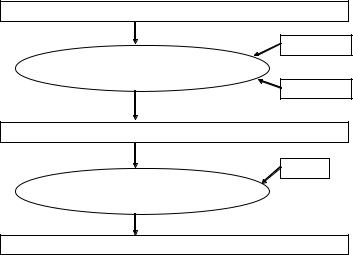
due to the bifurcations in the arteries of the plaqued vessels (see sections 9.6.1 and 9.6.2). Figure 9.23 illustrates the region merging algorithm. The input image has lumens which have one, two, or more classes. If the number of classes in the ROI is one class, then that class is selected; if two classes are in the ROI, then the minimum class is selected; and if there are three or more classes in the ROI, then the minimum two classes are selected. The selected classes are merged by assigning all the pixels of the selected classes one level value. This process results in the binarization of the left and right lumens.
The binary region labeling process is shown in Fig. 9.24. The process uses the CCA approach of top to bottom and left to right. Input is an image in which the lumen regions are binarized. The CCA first labels the image from the top to the bottom, and then from the left to the right. The result is an image that is labeled from the left to the right.
ID assignment process of the CCA for each pixel is shown in Fig. 9.25. In the CCA, in the input binary image, each white pixel is assigned a unique ID. The label propagation process then results in connected components. The propagation of