149 |
6.2 Riemannian manifolds |
Proof of the local-flatness theorem
Let {xα } be an arbitrary given coordinate system and {xα } the one which is desired: it reduces to the inertial system at a certain fixed point P. (A point in this four-dimensional manifold is, of course, an event.) Then there is some relation
xα = xα (xμ ),
α μ = ∂xα /∂xμ .
Expanding α μ in a Taylor series about P (whose coordinates are x0μ ) transformation at an arbitrary point x near P:
α μ (x) |
α μ ( |
P |
) |
+ |
(xγ |
− |
|
x0γ ) |
∂ α μ |
( |
P |
) |
|
|
|
|
|
|
∂xγ |
|
|
|
|
|
= |
|
|
|
|
|
|
|
|
|
|
|
|
|
|
|
|
|
|
|
|
|
|
|
|
|
1 |
|
|
|
γ |
|
|
|
|
|
|
γ |
|
|
|
λ |
|
|
|
|
|
|
λ |
|
|
∂2 α μ |
|
|
|
|
|
|
+ |
|
(x |
|
|
|
− x0 |
)(x |
|
|
|
− x0 ) |
|
(P) + · · · , |
|
|
2 |
|
|
|
|
∂xλ ∂xγ |
|
= α μ |P + (xγ − x0γ ) |
|
|
|
∂2xα |
|
|
* |
|
|
|
|
|
|
|
∂xγ |
∂xμ |
|
|
|
|
|
|
|
|
1 |
|
|
|
|
|
|
|
|
|
|
γ |
|
|
|
|
|
|
|
|
|
|
|
|
|
|
|
|
|
|
|
*3P |
α |
|
|
|
|
|
|
|
|
|
|
|
|
|
|
|
|
|
|
|
|
|
|
|
|
|
|
|
|
|
|
|
|
|
|
∂* |
x |
|
|
|
|
|
|
+ |
|
(xγ |
|
− |
x |
|
)(xλ |
|
− |
xλ ) |
|
|
|
|
|
* |
|
|
|
* |
+ · · · |
. |
|
2 |
|
|
|
∂xλ ∂xγ |
∂xμ |
|
|
|
|
|
|
|
|
|
0 |
|
|
|
|
|
|
0 |
|
|
|
|
|
|
|
|
|
|
|
|
|
|
|
|
|
|
|
|
|
|
|
|
|
|
|
|
|
|
|
|
|
|
|
|
|
|
|
|
|
*P |
|
|
|
|
|
|
|
|
|
|
|
|
|
|
|
|
|
|
|
|
|
|
|
|
|
|
|
|
|
|
|
|
|
|
|
|
|
|
|
|
* |
|
|
Expanding the metric in the same way gives |
|
|
|
|
|
|
|
|
|
|
* |
|
|
|
|
|
|
|
|
* |
|
|
|
|
|
|
|
|
|
|
|
|
|
|
|
|
|
|
|
|
γ |
) |
∂gαβ |
|
|
|
|
|
|
|
|
|
|
|
gαβ (x) = gαβ |P + (xγ − x0 |
|
|
|
|
|
|
|
|
|
|
|
|
|
|
∂xγ |
|
|
|
|
|
|
|
|
|
|
|
|
|
|
|
|
|
|
|
|
|
|
|
|
|
|
|
|
|
|
|
|
|
|
|
|
|
|
|
|
|
*P |
|
|
|
|
|
|
|
|
|
|
|
|
1 |
|
|
|
γ |
|
|
|
|
γ |
|
|
|
|
λ |
|
|
|
|
λ |
|
|
* |
|
∂2g |
αβ |
|
|
|
|
|
+ 2 (x |
|
|
|
|
)(x |
|
|
|
|
) |
* |
|
|
|
|
|
* |
+ · · · . |
|
|
|
|
− x0 |
|
|
|
− x0 |
|
∂xλ ∂xγ |
|
|
|
|
|
|
|
|
|
|
|
|
|
|
|
|
|
|
|
|
|
|
|
|
|
|
|
|
|
|
|
|
|
|
|
|
|
|
* |
|
|
|
|
|
|
|
|
|
|
|
|
|
|
|
|
|
|
|
|
|
|
|
|
|
|
|
|
|
|
|
|
|
|
|
|
|
|
|
|
*P |
|
|
|
|
|
|
|
|
|
|
|
|
|
|
|
|
|
|
|
|
|
|
|
|
|
|
|
|
|
|
|
|
|
|
|
|
|
|
|
|
* |
|
|
|
We put these into the transformation, |
|
|
|
|
|
|
|
|
|
|
|
|
|
|
|
|
|
|
|
|
|
|
|
|
|
* |
|
|
|
|
|
|
|
|
|
|
|
gu ν = α μ β ν gαβ , |
|
|
|
|
|
|
|
to obtain |
|
|
|
|
|
|
|
|
|
|
|
|
|
|
|
|
|
|
|
|
|
|
|
|
|
|
|
|
|
|
|
|
|
|
|
|
|
|
|
|
gμ ν |
(x) |
= |
α μ |
|P |
β ν |
|P |
gαβ |
|P |
|
|
|
|
|
|
|
|
|
|
|
|
|
|
|
|
|
|
|
|
|
|
|
|
|
|
|
|
|
|
|
|
|
|
|
|
|
|
|
|
+(xγ − x0γ )[ α μ |P β ν |Pgαβ,γ |P
+α μ |Pgαβ |P∂2xβ /∂xγ ∂xν |P
+β ν |Pgαβ |P∂2xα /∂xγ ∂xμ |P]
(6.21)
(6.22)
gives the
(6.23)
(6.24)
(6.25)
+ |
1 |
|
γ |
|
γ |
|
λ |
|
λ |
)[· · · ]. |
|
|
(x |
|
− x0 |
)(x |
|
− x0 |
(6.26) |
2 |
|
|
Now, we do not know the transformation, Eq. (6.21), but we can define it by its Taylor expansion. Let us count the number of free variables we have for this purpose. The matrixα μ |P has 16 numbers, all of which are freely specifiable. The array {∂2xα /∂xγ ∂xμ |P} has 4 × 10 = 40 free numbers (not 4 × 4 × 4, since it is symmetric in γ and μ ). The array {∂3xα /∂xλ ∂xγ ∂xμ |P} has 4 × 20 = 80 free variables, since symmetry on all
μ /∂xγ |P in Eq. (6.26) in
(6.29)
rearrangements of λ , γ and μ gives only 20 independent arrangements (the general expression for three indices is n(n + 1)(n + 2)/3!, where n is the number of values each index can take, four in our case). On the other hand, gαβ |P, gαβ,γ |P and gαβ,γ μ |P are all given initially. They have, respectively, 10, 10 × 4 = 40, and 10 × 10 = 100 independent numbers for a fully general metric. The first question is, can we satisfy Eq. (6.4),
gμ ν |P = ημ ν ? |
(6.27) |
This can be written as |
|
ημ ν = α μ |P β ν |Pgαβ |P. |
(6.28) |
By symmetry, these are ten equations, which for general matrices are independent. To satisfy them we have 16 free values in α μ |P. The equations can indeed, therefore, be satisfied, leaving six elements of α μ |P unspecified. These six correspond to the six degrees of freedom in the Lorentz transformations that preserve the form of the metric ημ ν . That is, we can boost by a velocity v (three free parameters) or rotate by an angle θ around a direction defined by two other angles. These add up to six degrees of freedom in α μ |P that leave the local inertial frame inertial.
The next question is, can we choose the 40 free numbers ∂ α such a way as to satisfy the 40 independent equations, Eq. (6.5),
gα β ,μ |P = 0?
Since 40 equals 40, the answer is yes, just barely. Given the matrix α μ |P, there is one and only one way to arrange the coordinates near P such that α μ ,γ |P has the right values to make gα β ,μ |P = 0. So there is no extra freedom other than that with which to make local Lorentz transformations.
The final question is, can we make this work at higher order? Can we find 80 numbersα μ ,γ λ |P which can make the 100 numbers gα β ,μ λ |P = 0? The answer, since 80 < 100, is no. There are, in the general metric, 20 ‘degrees of freedom’ among the second derivatives gα β ,μ λ |P. Since 100 − 80 = 20, there will be in general 20 components that cannot be made to vanish.
Therefore we see that a general metric is characterized at any point P not so much by its value at P (which can always be made to be ηαβ ), nor by its first derivatives there (which can be made zero), but by the 20 second derivatives there which in general cannot be made to vanish. These 20 numbers will be seen to be the independent components of a tensor which represents the curvature; this we shall show later. In a flat space, of course, all 20 vanish. In a general space they do not.
6.3 Co va r i a n t d i f f e re n t i a t i o n
We now look at the subject of differentiation. By definition, the derivative of a vector field involves the difference between vectors at two different points (in the limit as the points come together). In a curved space the notion of the difference between vectors at different
151 |
6.3 Covariant differentiation |
points must be handled with care, since in between the points the space is curved and the idea that vectors at the two points might point in the ‘same’ direction is fuzzy. However, the local flatness of the Riemannian manifold helps us out. We only need to compare vectors in the limit as they get infinitesimally close together, and we know that we can construct a coordinate system at any point which is as close to being flat as we would like in this same limit. So in a small region the manifold looks flat, and it is then natural to say that the derivative of a vector whose components are constant in this coordinate system is zero at that point. In particular, we say that the derivatives of the basis vectors of a locally inertial coordinate system are zero at P.
Let us emphasize that this is a definition of the covariant derivative. For us, its justification is in the physics: the local inertial frame is a frame in which everything is locally like SR, and in SR the derivatives of these basis vectors are zero. This definition immediately leads to the fact that in these coordinates at this point, the covariant derivative of a vector has components given by the partial derivatives of the components (that is, the Christoffel symbols vanish):
Vα :β = Vα .β at P in this frame. |
(6.30) |
This is of course also true for any other tensor, including the metric:
gαβ;γ = gαβ,γ = 0 at P.
(The second equality is just Eq. (6.5).) Now, the equation gαβ;γ = 0 is true in one frame (the locally inertial one), and is a valid tensor equation; therefore it is true in any basis:
gαβ:γ = 0 in any basis. |
(6.31) |
This is a very important result, and comes directly from our definition of the covariant derivative. Recalling § 5.4, we see that if we have μαβ = μβα , then Eq. (6.31) leads to Eq. (5.75) for any metric:
|
α |
1 |
αβ |
(gβμ,ν + gβν,μ − gμν,β ). |
|
|
μν = |
2 g |
|
(6.32) |
It is left to Exer. 5, § 6.9, to demonstrate, by repeating the flat-space argument now in the locally inertial frame, that μβα is indeed symmetric in any coordinate system, so that Eq. (6.32) is correct in any coordinates. We assumed at the start that at P in a locally inertial frame, α μν = 0. But, importantly, the derivatives of α μν at P in this frame are not all zero generally, since they involve gαβ,γ μ. This means that even though coordinates can be found in which α μν = 0 at a point, these symbols do not generally vanish elsewhere. This differs from flat space, where a coordinate system exists in which α μν = 0 everywhere. So we can see that at any given point, the difference between a general manifold and a flat one manifests itself in the derivatives of the Christoffel symbols.
Eq. (6.32) means that, given gαβ , we can calculate α μν everywhere. We can therefore calculate all covariant derivatives, given g. To review the formulas:
Vα ;β = Vα ,β + α μβ Vμ, |
(6.33) |
Pα;β = Pα,β − μαβ Pμ, |
(6.34) |
Tαβ ;γ = Tαβ ,γ + α μγ Tμβ + β μγ Tαμ. |
(6.35) |
|
|
Divergence formu la
Quite often we deal with the divergence of vectors. Given an arbitrary vector field Vα , its divergence is defined by Eq. (5.53),
|
Vα ;α = Vα ,α + α μα Vμ. |
(6.36) |
This formula involves a sum in the Christoffel symbol, which, from Eq. (6.32), is |
|
α μα = |
1 |
gαβ (gβμ,α |
+ gβα,μ − gμα,β ) |
|
|
|
2 |
|
|
1 |
gαβ (gβμ,α |
1 |
gαβ gαβ,μ. |
|
= |
|
− gμα,β ) + |
|
(6.37) |
2 |
2 |
This has had its terms rearranged to simplify it: notice that the term in parentheses is antisymmetric in α and β, while it is contracted on α and β with gαβ , which is symmetric. The first term therefore vanishes (see Exer. 26(a), § 3.10) and we find
|
α |
1 |
|
αβ |
|
|
|
μα = |
|
g |
|
gαβ,μ. |
(6.38) |
2 |
|
Since (gαβ ) is the inverse matrix of (gαβ ), it can be shown (see Exer. 7, § 6.9) that the derivative of the determinant g of the matrix (gαβ ) is
|
g,μ = ggαβ gβα,μ. |
|
|
|
(6.39) |
|
|
|
|
|
|
|
|
Using this in Eq. (6.38), we find |
|
|
|
|
|
|
|
|
|
|
|
α μα = (√ − g),μ/√ − g. |
|
|
(6.40) |
Then we can write the divergence, Eq. (6.36), as |
|
|
|
|
|
Vα |
Vα |
1 |
Vα (√ |
− |
g) |
|
(6.41) |
|
|
;α = |
,α + |
√ − g |
|
,α |
|
153 |
|
6.4 Parallel-transport , geodesics, and curvature |
|
|
|
|
|
|
|
|
|
|
|
or |
|
|
|
|
|
|
|
|
|
|
|
|
|
|
|
|
|
|
|
|
Vα ;α = |
√ |
1 |
g |
(√ − gVα ),α . |
(6.42) |
|
|
− |
|
|
|
|
|
|
|
|
|
|
|
|
|
|
|
This is a very much easier formula to use than Eq. (6.36). It is also important for Gauss’ law, where we integrate the divergence over a volume (using, of course, the proper volume element):
' Vα ;α √ − g d4x = ' (√ − gVα ),α d4x. |
(6.43) |
Since the final term involves simple partial derivatives, the mathematics of Gauss’ law applies to it, just as in SR (§ 4.8):
' (√ − gVα ),α d4x = ( Vα nα √ − g d3S. |
(6.44) |
This means
' Vα ;α √ − g d4x = ( Vα nα √ − g d3S. |
(6.45) |
So Gauss’ law does apply on a curved manifold, in the form given by Eq. (6.45). We need to integrate the divergence over proper volume and to use the proper surface element, nα √ − g d3S, in the surface integral.
6.4 Pa ra l l e l - t ra n s p o r t , g e o d e s i c s , a n d c u r va t u re
Until now, we have used the local-flatness theorem to develop as much mathematics on curved manifolds as possible without considering the curvature explicitly. Indeed, we have yet to give a precise mathematical definition of curvature. It is important to distinguish two different kinds of curvature: intrinsic and extrinsic. Consider, for example, a cylinder. Since a cylinder is round in one direction, we think of it as curved. This is its extrinsic curvature: the curvature it has in relation to the flat three-dimensional space it is part of. On the other hand, a cylinder can be made by rolling a flat piece of paper without tearing or crumpling it, so the intrinsic geometry is that of the original paper: it is flat. This means that the distance in the surface of the cylinder between any two points is the same as it was in the original paper; parallel lines remain parallel when continued; in fact, all of Euclid’s axioms hold for the surface of a cylinder. A two-dimensional ‘ant’ confined to that surface would decide it was flat; only its global topology is funny, in that going in a certain direction in a straight line brings him back to where he started. The intrinsic geometry of an n-dimensional manifold considers only the relationships between its points on paths that
remain in the manifold (for the cylinder, in the two-dimensional surface). The extrinsic curvature of the cylinder comes from considering it as a surface in a space of higher dimension, and asking about the curvature of lines that stay in the surface compared with ‘straight’ lines that go off it. So extrinsic curvature relies on the notion of a higher-dimensional space. In this book, when we talk about the curvature of spacetime, we talk about its intrinsic curvature, since it is clear that all world lines are confined to remain in spacetime. Whether or not there is a higher-dimensional space in which our four-dimensional space is an open question that is becoming more and more a subject of discussion within the framework of string theory. The only thing of interest in GR is the intrinsic geometry of spacetime.
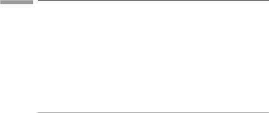
The cylinder, as we have just seen, is intrinsically flat; a sphere, on the other hand, has an intrinsically curved surface. To see this, consider Fig. 6.1, in which two neighboring lines begin at A and B perpendicular to the equator, and hence are parallel. When continued as locally straight lines they follow the arc of great circles, and the two lines meet at the pole P. Parallel lines, when continued, do not remain parallel, so the space is not flat.
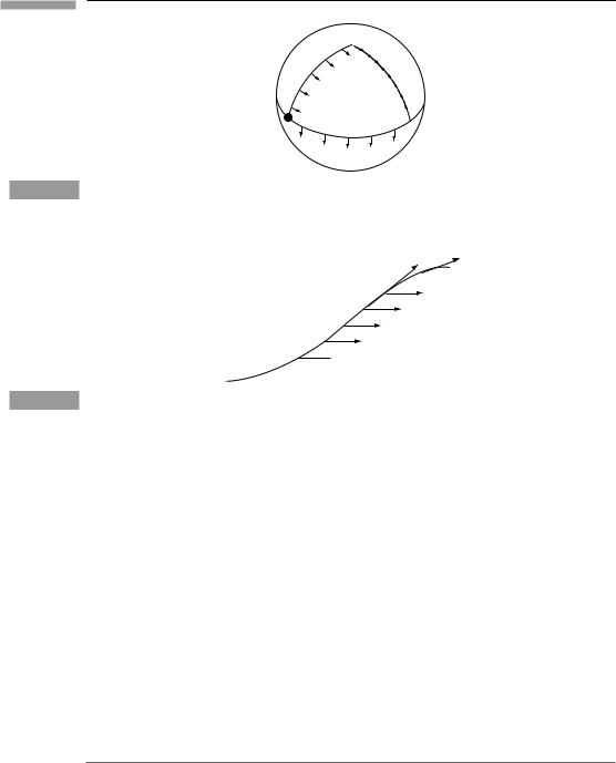
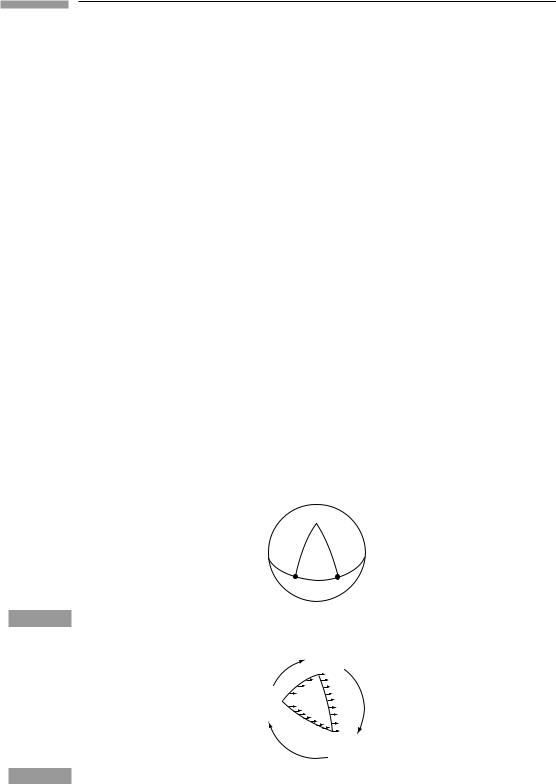
There is an even more striking illustration of the curvature of the sphere. Consider, first, flat space. In Fig. 6.2 a closed path in flat space is drawn, and, starting at A, at each point a vector is drawn parallel to the one at the previous point. This construction is carried around the loop from A to B to C and back to A. The vector finally drawn at A is, of course, parallel to the original one. A completely different thing happens on a sphere! Consider the path shown in Fig. 6.3. Remember, we are drawing the vector as it is seen to a twodimensional ant on the sphere, so it must always be tangent to the sphere. Aside from that, each vector is drawn as parallel as possible to the previous one. In this loop, A and C are on the equator 90◦ apart, and B is at the pole. Each arc is the arc of a great circle, and each is 90◦ long. At A we choose the vector parallel to the equator. As we move up toward B, each new vector is therefore drawn perpendicular to the arc AB. When we get to B,
 P
P
A B
A spherical triangle APB.
B
A 
C
A ‘triangle’ made of curved lines in flat space.
155
Figure 6.3
Figure 6.4
6.4 Parallel-transport , geodesics, and curvature
 B
B
A
C
Parallel transport around a spherical triangle.
→ →
U U
→
V
→
 V
V
Parallel transport of V along U.
the vectors are tangent to BC. So, going from B to C, we keep drawing tangents to BC. These are perpendicular to the equator at C, and so from C to A the new vectors remain perpendicular to the equator. Thus the vector field has rotated 90◦ in this construction! Despite the fact that each vector is drawn parallel to its neighbor, the closed loop has caused a discrepancy. Since this doesn’t happen in flat space, it must be an effect of the sphere’s curvature.
This result has radical implications: on a curved manifold it simply isn’t possible to define globally parallel vector fields. We can still define local parallelism, for instance how to move a vector from one point to another, keeping it parallel and of the same length. But the result of such ‘parallel transport’ from point A to point B depends on the path taken. We therefore cannot assert that a vector at A is or is not parallel to (or the same as) a certain vector at B.
Paral lel-transport
The construction we have just made on the sphere is called parallel-transport. Suppose a
vector field V is defined on the sphere, and we examine how it changes along a curve, as
in Fig. 6.4. If the vectors V at infinitesimally close points of the curve are parallel and of
equal length, then V is said to be parallel-transported along the curve. It is easy to write
=
down an equation for this. If U dx/dλ is the tangent to the curve (λ being the parameter