

Neutron Scattering in Biology - Fitter Gutberlet and Katsaras
.pdf16 Quasielastic Neutron Scattering: Applications |
357 |
Here, Ivib(Q, t), Irot(Q, t), Itrans(Q, t) are the incoherent intermediate and Svib(Q, ω), Srot(Q, ω), Strans(Q, ω) the incoherent Van Hove scattering functions of the three individual types of motions; the symbol stands for the convolution in energy transfer ω. The question, as to when this convolution approximation can be applied, requires some discussion. The vibrational term in this convolution can usually be replaced by a DWF, as long as the study is restricted to the quasielastic region. Strictly speaking, the independence approximation of rotational and translational motions is often invalid, for instance if the two motions are not occurring simultaneously and independently of each other, but as a sequence of alternating steps. The validity of the approximation is, however, recovered, if for instance the rate of rotational steps, Hrot, is much higher than the rate of translational steps, Htrans, because then it can be argued that the concerned particle is quasi-continuously participating in the rotational motion. Under the condition that the rates di er by at least an order of magnitude (a situation typical for many real systems), one can study the rotational motion “alone” in a low or medium resolution experiment, by choosing an intermediate energy resolution ∆( ω) such thatHtrans ∆( ω) ≤ Hrot. This simply means that the experimental observation time ∆tobs [4] (which in practice cannot be made infinite; see the related discussion in Sect. 15.2.3 of Part I in this volume) is larger than the build-up time of the local probability-density distribution (PDD)(for instance due to a reorientational motion), but much smaller than its time of decay due to long-range di usion. The elastic incoherent structure factor (EISF) ( [5] and [6]; see Sect. 15.2.2 of Part I in this volume) of the rotational motion can then be determined from the integral of the only weakly broadened elastic peak, whereas the rotation rate is obtained from the quasielastic line width of the broader spectral component. Vice versa translational di usion is studied alone in a high resolution experiment with ∆( ω) ≤ Htrans Hrot, because under this condition the rotational component will contribute only a flat background to the spectrum, whereas the di usion parameters can be determined from the Q-dependent line width of the central component of Ss(Q, ω). This has been the justification for applying the dynamic-independence approximation in many cases, e.g., for a number of superprotonic conductors exhibiting the Grotthuss mechanism [7–9]. The same principles are of course applicable in the case of biological studies.
16.3 The Gaussian Approximation
In early theoretical neutron scattering work, it had already been noticed [10] that in some idealized systems, such as the harmonic solid, the ideal gas and the particle di using according to the simple di usion equation or Langevin’s equation, Van Hove’s self-correlation function Gs(r, t) has a simple Gaussian shape in space. The Gaussian has also been employed in the case of less ideal systems, as a model for describing PDDs by elliptical (in 2D) or ellipsoidical

358 R.E. Lechner et al.
(in 3D) functions, with circle and sphere as special cases, respectively. In the isotropic case we have,
Gs(r, t) = (2πw(t))−3/2exp(−r2/2w(t)). |
(16.3) |
In reciprocal space, this is obviously reflected by Gaussian shapes in Q of the corresponding incoherent scattering functions, Is(Q, t) and Ss(Q, ω):
Is(Q, t) = exp − |
1 |
Q2w(t) , |
(16.4) |
||||
2 |
|||||||
|
+∞ |
|
|
1 |
|
|
|
Ss(Q, ω) = (2π)−1 |
exp − |
Q2w(t) e−iωtdt , |
(16.5) |
||||
|
|||||||
2 |
|||||||
−∞
where the function w(t) controls the time decay of Gs(r, t) and Is(Q, t) and is related to the energy width of Ss(Q, ω). In order to be able to explicitly calculate Ss(Q, ω) by carrying out this Fourier transformation, the (systemdependent) width function w(t) has to be specified. In the following, we give a few examples of Gaussian motion.
16.3.1 Simple Translational Di usion
In view of the omni-presence of water in living organisms, it is evident that atomic and molecular di usion play an important role in this context. It is worthwhile to start by considering the most simple di usion models, even if di usion processes in the interior of biological materials must be expected to be much more complex.2 Van Hove’s self-correlation function (accessible by incoherent neutron scattering, see Sect. 15.2.1 in Part I, this volume), in the case of simple (continuous) di usion is derived by solving the macroscopic di usion equation (e.g., in three dimensions), with the self-di usion coe cient
Ds,
∂Gs(r, t) |
= Ds 2Gs(r, t) , |
(16.6) |
∂t |
with the initial condition Gs(r, 0) = δ(r). The solution of this equation is well known. It is given by Eq. 16.3, if we write w(t) = 2Ds |t| for the width function. The corresponding intermediate scattering function is obtained by making the same substitution in Eq. 16.4. For the incoherent scattering function one obtains from Eq. 16.5 a simple Lorentzian with half-width at half-maximum
(HWHM) f (Q), |
f (Q)/π |
|
|
|
Ss(Q, ω) = |
, |
(16.7) |
||
|
||||
ω2 + f (Q)2 |
where f (Q) = DsQ2. We note, however, that this Gaussian behavior of the scattering functions is limited to the regime, where continuous di usion is a
2For a more general treatment of di usion studies employing quasielastic neutron scattering techniques, see [11]
16 Quasielastic Neutron Scattering: Applications |
359 |
valid picture, namely to su ciently low Q and long times. This corresponds to large displacements, where in general the di using particle is already far away from the origin (where it was at t = 0), and has “forgotten” where it came from and what the detailed structure of its neighborhood has been in the early stage of its journey. There is a number of other, more sophisticated, di usion models proposed by Chudley-Elliott [12], Singwi-Sj¨olander [13], Oskotskii [14], Egelsta [15], Rahman-Singwi-Sj¨olander [16], with Gaussian behavior for low Q and long times. Here, we can merely give reference to some of the original literature, but treat one of them [12] in some detail in Sect. 16.4.1, as a representative of noncontinuum di usion models taking account of the local structure. Another one (two-dimensional di usion) is discussed in Sect. 16.5.1.
16.3.2 Three-Dimensional Di usion of Protein Molecules in
Solution (Crowded Media)
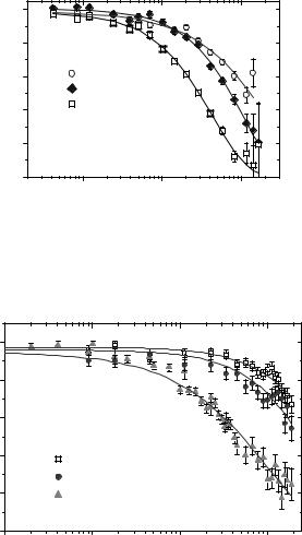
For studying the di usion of molecules as large as proteins in solution with fairly large concentrations, very high energy resolution is required, i.e., very large Fourier times must be reached. For this purpose, neutron spin-echo spectroscopy may be used to study such translational motions of proteins in solution under “crowded” conditions. As an example, we discuss an investigation of myoglobin solutions in vitro as a function of the protein volume fraction Φ 0.05–0.4 [17]. From a biological point of view, myoglobin is an oxygen storage molecule located in muscles and is believed to assist oxygen transport by di usion from the high oxygen partial pressure (near the cell membrane) to the low partial pressure regions (the mitochondria). Neutron scattering is the only technique which allows to study both protein interactions and protein motions over intermolecular distances at physiological concentration. In the case of NSE spectroscopy, it is advisable to use coherent neutron scattering (giving access to the Van Hove pair-correlation function, rather than to the self-correlation function). For this reason, and for maximizing the coherent scattering signal at small wave vectors, native hydrogeneous proteins are solved in D2O. Typical intermediate scattering functions measured on two di erent spectrometers are shown in Figs. 16.1 and 16.2. The relaxation function follows a single exponential decay and can be refined as
I(Q, t) = exp(−Dc(Q)Q2 |t|) . |
(16.8) |
Dc(Q) is an apparent collective di usion coe cient, close but not equal to the protein self-di usion coe cient, because a coherent quasielastic scattering function is measured. The precise interpretation of Dc(Q) in terms of self-di usion is not straight-forward. The wave vector and volume fraction dependence of Dc(Q) is plotted in Fig. 16.3. At large Q, Dc(Q) tends to a plateau value which corresponds to the short-time self-di usion coe cient sDs(Φ). This quantity is very strongly volume fraction dependent, although direct interactions are not relevant over such short distances (S(Q) 1 in
360 R.E. Lechner et al.
|
1.0 |
|
|
|
t, =0) |
0.8 |
|
|
|
0.6 |
Q=0.076 Å−1 |
|
||
(Q |
|
Q=0.120 Å−1 |
|
|
t)/I |
0.4 |
Q=0.207 Å−1 |
|
|
, |
|
|
|
|
I(Q |
|
|
|
|
|
Myoglobin 14.7mM + D2O |
|
||
|
0.2 |
|
||
|
|
TS = 37˚C |
|
|
|
0.0 |
100 |
1000 |
10000 |
|
|
|||
|
|
|
spin echo time t [ps] |
|
Fig. 16.1. Intermediate scattering function of 14.7 mM myoglobin solution in D2O, as obtained with the spectrometer MUSES [18] at LLB, Saclay. The instrument was used in its NSE mode of operation (see Sect. 15.4 in Part I, this volume), at three di erent wavevectors around the structure factor maximum (from [17])
|
1.0 |
|
|
|
=0) |
0.8 |
|
|
|
|
|
|
|
|
(Q,t |
0.6 |
Myoglobin 30mM |
|
|
|
|
|
||
)/I |
|
|
|
|
|
|
|
|
|
(Q,t |
0.4 |
Q =0.02Å−1 |
|
|
I |
|
Q =0.04Å−1 |
|
|
|
|
|
|
|
|
0.2 |
Q =0.08Å−1 |
|
|
|
0.0 |
|
|
|
|
102 |
103 |
104 |
105 |
spin echo time t [ps]
Fig. 16.2. Intermediate scattering function of 30 mM myoglobin solution in D2O, as obtained with the NSE spectrometer IN15 at ILL, Grenoble (see Sect. 15.4 in Part I, this volume), for three di erent wavevectors in the very low Q-range (from [17])
this wave vector range). Hydrodynamic interactions are responsible for this strong volume dependence. At smaller wave vectors Dc(Q) increases. It probes pair-correlation relaxations which are accelerated by concentration fluctuation relaxations. In the limit of Q 0,
Dc = |
1 ∂Π |
, |
(16.9) |
|||
|
|
|
||||
f ∂C |
||||||
|
|
|
||||
16 Quasielastic Neutron Scattering: Applications |
361 |
|
0.14 |
|
Myoglobin |
|
14.7mM : φ=0.18 |
|
|
|
|
|
|||
|
0.12 |
|
|
|
21.7mM : φ=0.28 |
|
1 |
|
|
|
|
30.0mM : φ=0.4 |
|
− |
|
|
|
|
|
|
s |
0.10 |
|
|
|
|
|
2 |
|
|
|
|
|
|
cm |
0.08 |
|
|
|
|
|
−5 |
|
|
|
|
|
|
)10 |
0.06 |
|
|
|
|
|
Q( |
|
|
|
|
|
|
|
|
|
|
|
|
|
c |
|
|
|
|
|
|
D |
0.04 |
|
|
|
|
|
|
|
|
|
|
|
|
|
0.02 |
|
|
|
|
|
|
0.00 |
|
|
|
|
|
|
0.00 |
0.05 |
0.10 |
0.15 |
0.20 |
0.25 |
|
|
|
wavevector Q (A−1) |
|
||
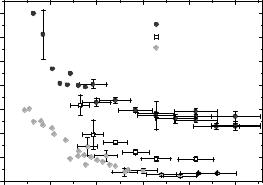
Fig. 16.3. Apparent collective di usion coe cient Dc(Q) of myoglobin in D2O solution, for three di erent concentrations. The wavevector dependence exhibits a plateau at large Q, related to the short-time self-di usion coe cient sDs(Φ). Electrostatic interaction is responsible for the increase at small Q (from [17])
where f is a friction coe cient and ∂Π is the reciprocal osmotic compress-
∂C
ibility which acts as a force tending to relax the concentration fluctuations. Generally such studies combined with an analysis of the small-angle neutron scattering (SANS) spectra in terms of direct protein–protein interactions allow to separate hydrodynamic and direct interactions [19]. An interesting property of QENS is that it allows to probe protein dynamics directly inside cells as for example in the case of hemoglobin in red blood cells [20].
16.3.3 Vibrational Motions, Phonon-Expansion and Debye–Waller factor (DWF), Dynamic Susceptibility
In solids, atoms, and molecules perform vibrations around fixed equilibrium positions and orientations. The frequency spectrum of these vibrations is described by the phonon density of states g(ω). In the simplest case of a long-range ordered crystalline system (cubic crystal in the harmonic approximation, with only one atom per unit cell), the wave-like propagation of vibrations is exactly represented by the scattering function Svib(Q, ω), in the form of the phonon-expansion [21, 22]:
2 2 |
∞ |
|
< u2 > Q2 |
|
n |
|
|
|
|
|
|
|
|
|
|
|
|
Svib(Q, ω) = e−<u >Q |
δ(ω) + |
|
n! |
|
|
Sn(ω) |
, |
(16.10) |
|
n=1 |
|
|
|
|
|
||
where <u2> is the atomic mean square displacement and e−<u2>Q2 is the DWF. The latter obviously stands for the Gaussian behavior in space of
362 R.E. Lechner et al.
the time-averaged atomic probability density distribution in the harmonic solid. The first term of the sum, δ(ω), represents the purely elastic scattering, while the terms Sn(ω) correspond to n-phonon transitions. The normalized one-phonon term S1(ω) is the product of the Bose phonon-population factor nB(ω, T ) with g(ω),
S1(ω) = nB(ω, T )g(ω) , |
(16.11) |
|||||
nB(ω, T ) = |
1 |
|
, |
(16.12) |
||
|
|
|
|
|||
|
ω |
|
||||
|
e |
kBT |
|
− 1 |
|
|
where T is the temperature, kB and are the Boltzmann and Planck constants, respectively. Equation 16.12, can also be written in the following form:
nB(ω, T ) = exp(− ω/2kBT ) [2ω sinh( ω/2kBT )]−1 |
(16.13) |
Note that now the detailed balance factor, exp(− ω/2kBT ) appears explicitly in this expression (compare Eqs. 16.18 to 16.20, Sect. 15.2.1 in Part I, this volume). Each profile Sn(ω) (n ≥ 1) is obtained by folding S1(ω) (n − 1) times with itself. Since the detailed-balance factor is invariant against this convolution, it can in practice be extracted from the convolution kernel and put in front of the sum in Eq. 16.10. The normalization of the incoherent scattering function 16.10 follows from the definition:
∞
S1(ω)dω = 1 , |
(16.14) |
−∞
and therefore
∞
Sn(ω)dω = 1 , |
(16.15) |
−∞
for all n. In the presence of motions with a di usive character, in addition to vibrations, the scattering function will also have a quasielastic component that may be combined with the vibrational component 16.10 according to the dynamic independence approximation 16.2, where applicable. If quasielastic scattering is inexistent or unresolved, e.g., in experiments limited to low temperatures (T ≤ 100 K) and/or to large or medium energy resolution widths (∆( ω) ≥ 90 meV), observed inelastic neutron scattering spectra will be due to vibrational excitations only.
In biological matter, e.g., proteins, the spatial arrangement of atoms and the dynamics are much more complex, than in the above-mentioned type of systems with long-range crystalline order. The unperturbed spatial propagation of vibrational modes is then typically restricted to shorter ranges. An exact theory is usually intractable. But, for practical purposes, we may employ expression 16.10 to extract an e ective vibrational density of states from measured neutron scattering spectra. This is a rather useful semiphenomenological quantity, especially in studies of the evolution of vibrational dynamics as a function of external parameters. The e ective density of states
16 Quasielastic Neutron Scattering: Applications |
363 |
g(ω) accounts for the individual displacement amplitudes, phonon polarization vectors, and masses of the ensemble of generalized oscillators of the complex protein system. For small values of <u2> and Q2 the higher order terms in 16.10 can be neglected, i.e., a one-phonon approximation may be employed, where Eq. 16.10 reduces to
Svib(Q, ω) = e−<u2>Q2 δ(ω)+ < u2 > Q2S1(ω) . |
(16.16) |
The e ective vibrational density of states can be determined using the above expressions in either one of the following two ways: (i) Svib(Q, ω) according to Eqs. 16.10 and 16.11, is fitted to the spectra measured over an extended Q-range, using suitable model functions for g(ω), or (ii) g(ω) is found, independently of model functions, by taking the inelastic part of the measured data to the limit
g(ω) = Q→0 |
Q2 |
B |
− |
|
vib |
|
|
|
lim |
|
2M |
[n (ω, T )] |
|
1S |
|
(Q, ω) , |
(16.17) |
|
|
|
|
|||||
where M is the e ective molecular mass. The second procedure has sometimes been applied, even when the dynamics of the system under study is not governed exclusively by harmonic or quasiharmonic vibrations. When strongly damped, overdamped or almost purely stochastic motions are also present, the function g(ω) then obtained by this method, obviously is a “generalized” one, in the sense that it also includes the e ects of those additional motions. Their signature is, that the generalized function does not show the ω2-behavior wellknown for harmonic vibrations at low energies, and starts with a finite value at ω = 0 (see Sect. 16.4.4).
Instead of the Van Hove scattering functions the corresponding dynamic susceptibilities are sometimes used. The susceptibility χ(Q, ω) is defined in the framework of linear response theory [23] as the steady state response of a system to an oscillatory force. In other words, it corresponds to nontransient response and defines the fluctuations in the unperturbed system. The function,
χ(ω) = χ (ω) + iχ (ω) , |
(16.18) |
is a complex quantity; the real part corresponds to the in-phase and the imaginary part to the out-of-phase response. The fluctuation–dissipation theorem describes, how fluctuations of the system will be dissipated in it at thermal equilibrium. χ (Q, ω) is related to the dynamic structure factor (i.e., the scattering function):
S(Q, ω) = nB(ω, T )χ (ω). |
(16.19) |
Using the imaginary part of the dynamic susceptibility can be particularly useful in some special cases: for instance, in the case of a simple harmonic oscillator and equally for purely harmonic crystals, χ (Q, ω) does not depend on temperature, because here all the temperature e ect is contained in the Bose phonon-population factor nB(ω, T ). χ (Q, ω) is consequently sometimes used to study those e ects which do not depend on thermal population.

364 R.E. Lechner et al.
16.3.4 Vibrational Density of States of the Light-harvesting Complex II of Green Plants
Photosynthesis is a fundamental physiological process in nature representing the transformation of solar radiation into storable chemical energy. One of the important functions of antenna complexes during the primary steps of photosynthesis, is to perform an e cient excitation energy transfer (EET) to photoactive pigments bound in the “reaction center” complexes (for reviews see [24] and [25]). The major antenna complex of green plants is the light-harvesting complex of photosystem II (LHC II) (for a review see [26]). Apart from the energy level structure of the excited electronic states [27–29], the coupling of the purely electronic transitions of pigments to intramolecular and low-frequency vibrational modes of the protein matrix (“electronphonon” coupling3) plays an essential role in light absorption and ultrafast EET [30,31] (for a review see [32]). Because of this coupling and the broadening of electronic states resulting from it, the energy transfer between electronic states of neighboring pigments is facilitated and e ectively mediated by the protein matrix’s vibrational density of states. A knowledge of the latter is required for the calculation of energy transfer rates. In view of the inherent complexity of the interpretation of phonon structure obtained from optical spectroscopy (hole-burning (HB) and fluorescence line-narrowing (FLN) spectra [33]), inelastic incoherent neutron scattering (IINS) has become a technique of choice as an independent experimental approach to study the vibrational density of states of photosynthetic pigment–protein complexes.
IINS spectra of proteins generally display a peak centered at energy transfers somewhere in the range from 2 to 5 meV, representing an excess of vibrational modes, as compared to the low-frequency region of a Debye-like density of states. The origin of this so-called “Boson peak” known to be characteristic for both, proteins and glassy systems [34–39], is not yet fully understood, but it is believed to be related to the disordered nature of these systems. The e ective density of states derived from IINS spectra (see e.g., [34, 37]), which is of a fundamental interest in itself, also permits a comparison to molecular dynamics (MD) simulations of internal protein motions (see e.g., [40]). Here, we discuss results of IINS experiments on the photosynthetic antenna complex LHC II from spinach [41]. Trimeric LHC II was solubilized in a D2O containing bu er solution, so that the solvent scattering was significantly
3In the present context, the term “phonon” is largely employed, when referring to low-frequency protein vibrations (<25 meV). This is customary in studies of pigment–protein complexes in order to distinguish such modes from higher-frequency vibrational modes of the pigment molecules (60–250 meV). However, in biological systems one is generally not dealing with phonons in a rigorous sense. Due to lack of long-range order, vibrational modes, except for long-wavelength sound waves, are expected to travel only over short distances before they are seriously damped
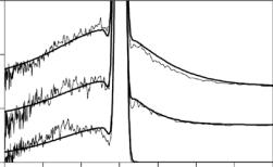
 80K
80K