Neutron Scattering in Biology - Fitter Gutberlet and Katsaras

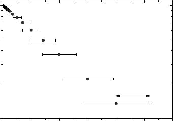
348 R.E. Lechner et al.

spin−echo time τ [ps]

Fig. 15.12. Logarithmical plot of an exponentially decaying intermediate scattering function, I(Q, t), on a linear time-scale, showing typical spin–echo time integration windows of a spin–echo spectrometer with a velocity selector selecting a wavelength band with ∆λ0/λ0 0.15 (FWHM). The horizontal bars represent the standard deviation σ of the spin–echo time τ

NSE spectroscopy is often used for the measurement of slowly decaying relaxation functions. In such cases, the consequence of such broad time integration windows is sometimes of little importance and usually neglected.

15.5 Miscellaneous Technical Points:

MSC, Calibration, Contrast

Let us finally mention a few technical points concerning the analysis of data originating from QENS experiments. At first, we consider those aiming at the direct determination of Van Hove’s scattering functions in (momentum, energy)-space. An important problem in the evaluation of quasielastic neutron scattering spectra is the accurate consideration of the experimental resolution. Although straightforward, this is complex, if the spectrum is a sum of several quasielastic components, eventually superimposed by a purely elastic line, either due to the fact that the di usive motion is localized, or caused by parasitic incoherent scattering from the host material in which the particles perform a di usive motion. The measured spectra are convolutions of the scattering function with the resolution function. Since a direct deconvolution generally encounters practical di culties, in a typical analysis the data are usually not directly corrected for resolution, but an inverse procedure is employed. It consists in folding the theoretical model with the measured

resolution function and comparing the result to the measured spectra via nonlinear least-squares fitting calculations. This method, which amounts to an indirect deconvolution, is well-known, and standard software packages are available in the neutron scattering centers.

Another problem is multiple scattering (MSC). In principle, a neutron reaching the detector, may have been scattered in the sample once , twice, or even several times. For a given nominal scattering angle ϕ or nominal

Q value (Q (4π/λ) sin(ϕ/2)) the weighted double-, triple-,. . . scattering

=

spectra are then superimposed on the single-scattering data. The MSC components should be minimized by using su ciently thin samples. It is usually assumed that a reasonable sample thickness (a compromise between maximizing single-scattering of neutrons and minimizing the contribution of multiple to total scattering) should correspond to a transmission of T 0.9 (roughly 10% of the incident beam is scattered once and about 1% more than once). This leads for example to about 0.2 mm thickness for λ = 5 ˚A in the case of light water and to about 2 mm for deuterated water. Nevertheless, each case should be carefully studied especially with respect to sample absorption and geometry. A numerical correction is often necessary. Analytical methods [77] directly applied to the theoretical models, and model-independent MonteCarlo techniques (see for instance [78, 79]) are employed for this purpose. For the multiple scattering correction of NSE experiments, the same principles as already described apply, except that this has to be applied in the time domain, where instead of the deconvolution a simple division by the observation function has to be performed.

The third problem is calibration, which means the absolute determination of the scattered intensity, instead of quoting “arbitrary units”. Calibration is performed, for instance, by comparing the scattered intensity of a sample to that of a vanadium scatterer which has the same scattering geometry as the sample itself, and whose incoherent scattering cross-section is well-known (provided that there is no hydrogen contamination). In NSE experiments, usually a relative intensity normalization of the measured intermediate scattering function I(Q, t) is performed. For each spin–echo time, the measured polarization is divided by the polarization measured at τ = 0 (i.e., determined without a magnetic field in the coils). Theoretically, I(Q, τ = 0) should be equal to S(Q) = −∞∞ S(Q, ω)dω, but due to the fact that the spectrometer transmits only a wavelength band with a limited width, the integral over the scattering function remains incomplete. If a significant amount of the scattered intensity is outside of the spectrometer window, the normalization will therefore not be absolute. For an absolute calibration the required structure factor S(Q) of the sample must be determined independently, for practical reasons on a di erent instrument which does not have such a limited bandwidth transmission.

For many elements coherent and incoherent scattering coexists, and it is di cult to separate the contributions S(Q, ω) and Ss(Q, ω). Spin-incoherent scattering causes a fraction of (2/3)[σinc/(σinc + σcoh)] of the neutrons to flip

of scattering functions and correlation functions, elastic and quasielastic incoherent structure factors have been treated, and the importance of energy resolution and observation time and their variation have been emphasized. A number of selected instruments have been described, which are representative for di erent ranges of momentum transfer Q, energy transfer ω, and energy resolution ∆ ω, or Fourier time t and observation time ∆tobs. While, in principle, all types of instrument can cover the same or similar Q-ranges depending on the incident neutron wavelength, this is not so for ω, ∆ ω, t, and ∆tobs. Moderate, high and very high energy resolution are provided by time-of-flight, backscattering and spin–echo techniques, respectively. There is however appreciable overlap between the resolution ranges of di erent instruments, and this is beneficial, since results from di erent instruments must often be combined. Furthermore, it is also important to realize, that – because molecular motions occur on time-scales extending over many orders of magnitude – the access to every possible resolution is required, i.e., there is no “bad resolution”. As a consequence, the application of observation-time dependent quasielastic neutron scattering, in order to investigate dynamic e ects due to di usive atomic and molecular motions has been rapidly expanding and has a very promising future. The high intensities available at modern neutron scattering instruments and especially in the near future at the high-power spallation neutron sources now under construction, will allow the systematic experimental study of such motions on time scales extending over six orders of magnitude at least, and as a function of external parameters.

Regarding the problem, which instrument to choose for a given task, or which spectrometer to start with, it is clear that the relevant temporal and spatial scales are the first criteria to be considered. There are also some general remarks to be made: Once the scale question has been settled, one must decide, whether it is better to employ a (Q, ω)- or a (Q, t)-instrument. Spectrometers working in (Q, ω)-space are more e cient for the study of small quasielastic or inelastic e ects in the presence of large elastic components. The reason is, that under conditions of su cient energy resolution, elastic, and nonelastic phenomena are experimentally well separated, whereas in the case of (Q, t)-techniques the elastic term of the scattering function leads to a time-independent (possibly large) “elastic” background underneath the timedependent relaxation function to be studied. Without this problem, i.e., when the elastic component is small or absent, (Q, t)-instruments are very well suited, especially if rather long Fourier times are required. Furthermore, it is known that the latter techniques are generally more suitable for coherent than for spin-incoherent scattering, because the spin-flip scattering component reduces the useful intensity and can appreciably deteriorate the signal-to- noise ratio. The detailed performance (spectral and reciprocal-space regions, i.e., time and energy domains, momentum-transfer ranges, measurement e - ciency) of the di erent QENS techniques, TOF, BSC, NSE, NRSE, in various experimental situations, is best appreciated by comparing di erent experimental results (for a few examples, see Part II in this volume). The question,

352 R.E. Lechner et al.

how to make best use of the complementarity of the di erent techniques, in order to obtain a maximum of information, must be addressed systematically on the basis of such a comparison before any experimental study.

References

1.L. Van Hove, Phys. Rev. 95, 249 (1954)

2.S.W. Lovesey, Theory of Neutron Scattering from Condensed Matter (Clarendon Press, Oxford, 1984)

3.G.L. Squires, Introduction to the Theory of Thermal Neutron Scattering (University Press, Cambridge, 1978)

4.M. B´ee, Quasielastic Neutron Scattering: Principles and Applications in Solid State Chemistry, Biology and Materials Science (Adam Hilger, Bristol, 1988)

5.L. Koester, H. Rauch, E. Seymann, At. Data Nucl. Data Tables 49, 65 (1991)

6.V.F. Sears, Phys. Rep. 82, 1 (1982)

7.H. Stiller, in Inelastic Scattering of Neutrons, Vol. 2 (IAEA Vienna, 1965) p. 179

8.K. Sk¨old, J. Chem. Phys. 49, 2443 (1968)

9.A.J. Leadbetter, R.E. Lechner, in The Plastically Crystalline State, J.N. Sherwood (Eds.) (J. Wiley and Sons, New York, 1979) pp. 285–320

10.R.E. Lechner, in Quasielastic Neutron Scattering, J. Colmenero, A. Alegr´ıa, F.J. Bermejo (Eds.), Proceedings of the Quasielastic Neutron Scattering Workshop QENS’93, San Sebasti´an, Spain 1993 (World Scientific, Singapore, 1994)

pp.62–92

11.M. B´ee, Chem. Phys. 292, 121 (2003)

12.A.J. Dianoux, F. Volino, H. Hervet, Mol. Phys. 30, 1181–1194 (1975)

13.V.F. Sears, Can. J. Phys. 45, 237 (1967)

14.F. Volino, A.J. Dianoux, Mol. Phys. 41, 271 (1980)

15.R.E. Lechner, in Mass Transport in Solids, F. Beni`ere, C.R.A. Catlow (Eds.), NATO ASI (1981: Lannion, France) Series B: Physics, Vol. 97 (Plenum Publ. Corp. New York, 1983) pp. 169–226.

16.J. Fitter, R.E. Lechner, G. B¨uldt, N.A. Dencher, Proc. Natl. Acad. Sci. USA 93, 7600–7605 (1996)

17.T. Springer, Quasielastic Neutron Scattering for the Investigation of Di u- sive Motions in Solids Liquids, Springer Tracts in Modern Physics, Vol. 64 (Springer-Verlag, Berlin, 1972)

18.R.E. Lechner, Physica B 301, 83–93 (2001)

19.B. Ru ´e, J. Ollivier, S. Longeville, R.E. Lechner, Nucl. Instr. Methods A 449, 322 (2000)

20.D.L. Price, K. Sk¨old, Neutron Scattering, Methods of Experimental Physics, Vol. 23, part B, Chapters 8–11 (Academic Press, London, 1987)

21.R.E. Lechner, C. Riekel, in Neutron Scattering and Muon Spin Rotation, Springer Tracts in Modern Physics, Vol. 101, (Springer-Verlag, Berlin, 1983)

pp.1–84

22.D. Richter, in Neutron Scattering and Muon Spin Rotation, Springer Tracts in Modern Physics, Vol. 101 (Springer-Verlag, Berlin, 1983) pp. 85–222

23.S.W. Lovesey, T. Springer, Dynamics of Solids and Liquids by Neutron Scattering, Topics in Current Physics, Vol. 3 (Springer-Verlag, Berlin, 1977)

24.T. Springer, R.E. Lechner, in Di usion in Condensed Matter, P. Heitjans, J. K¨arger (Eds.) (Springer Verlag, Berlin, Heidelberg, 2005) pp. 93–164

25.C.G. Windsor, Pulsed Neutron Scattering (Taylor & Francis, London, 1981)

26.R. Scherm, C. Carlile, A.J. Dianoux, J. Suck, J. White, ILL Int. Rep. 76S235, (1976)

27.Y. Blanc, ILL Int. Rep. 83BL21G, (1983)

28.see http://www.ill.fr/YellowBook/IN6/

29.J. Mesot, S. Janssen, L. Holitzner, R. Hempelmann, J. Neutron Res. 3, 293– 310 (1996)

30.H. Mutka, Nucl. Instr. Methods Phys. Res. A, 338, 144–150 (1994)

31. R.E. Lechner, in Proceedings of ICANS-XV Conference, Tsukuba, 2000,

J.Suzuki, S. Itoh (Eds.) (JAERI, Tokai-mura, Japan, 2001) pp. 357–376

32.R.E. Lechner, in Neutron Scattering in the ’Nineties (IAEA, Vienna, 1985) pp. 401–407

33.R. Scherm, Int. Rep., KFA J¨ulich, (1965) J¨ul-295-NP

34.F. Douchin, R.E. Lechner, Y. Blanc, Int. Tech. Rep. ITR, ILL Grenoble 26, 73 (1973)

35.J. Ollivier, H. Casalta, H. Schober, J.C. Cook, P. Malbert, M. Locatelli,

C.Gomez, S. Jenkins, I.J. Sutton, M. Thomas, Appl. Phys. A 74, [Suppl.] S305–S307 (2002)

36.J. Ollivier, M. Plazanet, H. Schober, J.C. Cook, Physica B 350, 173–177 (2004)

37.S. Hautecler, E. Legrand, L. Vansteelandt, P. d’Hooghe, G. Rooms, A. Seeger,

W.Schalt, G. Gobert, in Neutron Scattering in the ’Nineties (IAEA, Vienna, 1985) pp. 211

38.R.E. Lechner, in Proceedings of ICANS-XI, KEK Report 90–25, M. Misawa, M.Furusaka, H. Ikeda, N. Watanabe (Eds.) (National Laboratory for HighEnergy Physics, Tsukuba, March 1991) pp. 717–732

39.R.E. Lechner, Physica B 180 & 181, 973 (1992)

40.R.E. Lechner, Neutron News 7, 9 (1996)

41.R.E. Lechner, R. Melzer, J. Fitter, Physica B 226, 86 (1996)

42.J.R.D. Copley, Nucl. Instr. Methods A 291, 519–532 (1990)

43.J.G. Smit, H. Dachs, R.E. Lechner, Solid State Commun. 29, 219–223 (1979)

44.R.E. Lechner, Appl. Phys. A 74, [Suppl.] S151 (2002)

45.B. Alefeld, M. Birr, A. Heidemann, Naturwissenschaften 56, 410 (1969)

46.B. Alefeld, T. Springer, A. Heidemann, Nucl. Sci. Eng. 110, 84 (1992)

47.B. Frick, A. Magerl, Y. Blanc, R. Rebesco, Physica B 234–236, 1177 (1997)

48.B. Frick, Neutron News 13, 15 (2002)

49.H. Rauch, in Neutron Di raction, H. Dachs (Eds.) Topics in Modern. Physics, Vol. 6 (Springer-Verlag, Berlin, 1978)

50.C.G. Shull, N.S. Ginrich, J. Appl. Phys. 35, 678 (1964)

51.P.M. Gehring, D.A. Neumann, Physica B 241–243, 64–70 (1998)

52.A.J. Dianoux, Physica B 182, 389 (1992)

53.A. Kollmar, B. Alefeld, in Proceedings of the Conference on Neutron Scattering, Gatlinburg, Tenn. USA 1976, R.M. Moon (Eds.), (National Techn. Information Service, US Dept. Of Comm., Springfield, 1976) pp. 330–336.

54.M. Prager, W. Press, B. Alefeld, A. H¨uller, J. Chem. Phys. 67, 5126 (1977)

55.G.P. Singh, F. Parak, S. Hunklinger, K. Dransfeld, Phys. Rev. Lett. 47, 685– 688 (1981)

56.F. Parak, E.W. Knapp, D. Kucheida, J. Mol. Biol. 161, 177–194 (1982)

354R.E. Lechner et al.

57.F. Parak, in Biomembranes, Methods in Enzymology, Vol. 127, L. Packer (Eds.) (Academic Press, Inc. London, 1986) pp. 197–206.

58.W. Doster, S. Cusack, W. Petry, Nature 337, 754–758 (1989)

59.W. Doster, S. Cusack, W. Petry, Phys. Rev. Lett. 65, 1080–1083 (1990)

60.R.E. Lechner, H.-J. Bleif, H. Dachs, R. Marx, M. Stahn, Solid, State Ionics 46, 25 (1991)

61.C.J. Carlile, M.A. Adams, Physica B 182, 431–440 (1992)

62.R.W. Connaster Jr., H. Belch, L. Jirik, D.J. Leach, F.R. Trouw, J.-M. Zanotti, Y. Ren, R.K. Crawford, J.M. Carpenter, D.L. Price, C.-K. Loong, J.P. Hodges, K.W. Herwig, in Proceedings of ICANS-XVI Conference, D¨usseldorf-Neuss, 2003, G. Mank, H. Conrad (Eds.) (FZ J¨ulich, Germany, 2003) pp. 279–288

63.W. Doster, M. Diehl, W. Petry, M. Ferrand, Physica B 301, 65 (2001)

64.W. Doster, M. Diehl, R. Gebhardt, R.E. Lechner, J. Pieper, Chem. Phys. 292, 487–494 (2003)

65.F. Mezei, Z. Physik 255, 146–160 (1972)

66.F. Mezei, Neutron Spin Echo, Lecture Notes in Physics Vol. 128 (Springer Verlag, Berlin, 1980)

67.C. Cohen-Tannoudji, B. Diu, F. Lalo¨e, M´ecanique Quantique I (Hermann ed., Paris, 1977)

68.R.P. Feynman, The Feynman Lectures on Physics, Quantum Mechanics (Addison-Wesley, 1965)

69.J.B. Hayter, Z. Physik B 31, 117–125 (1978)

70.J.B. Hayter, J. Penfold, Z. Physik B 35, 199–205 (1979)

71. O. Sch¨arpf, in Neutron Spin Echo, Lecture Notes in Physics Vol. 128,

F. Mezei (Eds.) (Springer Verlag, Berlin, 1980) pp. 27–52

72.J.B. Hayter, in Neutron Spin Echo, Lecture Notes in Physics Vol. 128,

F.Mezei (Eds.) (Springer Verlag, Berlin, 1980) pp. 53–65

73.F. Mezei, in Coherence and Imaging Processes in Physics, M. Schlenker, M. Fink, J.P. Goedgebuer, C. Malgrange, J.C. Vienot, R.H. Wade (Eds.), Vol. 112 (Springer-Verlag, Les Houches, 1979) pp. 282–295

74.S. Longeville, W. Doster, M. Diehl, R. G¨ahler, W. Petry, in Neutron SpinEcho Spectroscopy, Lecture Notes in Physics, Vol. 601, F. Mezei, C. Pappas,

T.Gutberlet (eds.) (Springer-Verlag, Berlin, 2003) pp. 325–335

75.R. G¨ahler, R. Golub, Z. Physik B – Condens. Matter 65 269–273, (1987)

76.R. Golub, R. G¨ahler, Phys. Lett. A, 123 43–48, (1987)

77.V.F. Sears, Adv. Phys. 24, 1 (1975)

78.R.E. Lechner, G. Badurek, A.J. Dianoux, H. Hervet, F. Volino, J. Chem. Phys. 73, 934 (1980)

79.M. Russina, F. Mezei, R.E. Lechner, S. Longeville, B. Urban, Phys. Rev. Lett. 84, 3630 (2000)

80.C. Lamers, O. Sch¨arpf, W. Schweika, J. Batoulis, K. Sommer, D. Richter, Physica B 180 & 181, 515 (1992)

81.J.C. Cook, D. Richter, O. Sch¨arpf, M.J. Benham, D.K. Ross, R. Hempelmann, I.S. Anderson, S.K. Sinha, J. Phys. Condens. Matter 2, 79 (1990)

16

Quasielastic Neutron Scattering in Biology,

Part II: Applications

R.E. Lechner, S. Longeville

16.1 Introduction

Low-frequency harmonic, damped harmonic, anharmonic, localized di usive (stochastic) translational, and rotational motions of biological macromolecules or of molecular subunits, are an important part of the dynamical characteristics of biological matter. They are believed to be essential for biological function. The ensemble of low-energy transfer inelastic (IENS) and quasielastic neutron scattering (QENS1) techniques, is particularly well-suited for the investigation of dynamic structure. The instrumentation and the basic theory have been treated in Part I in this volume. The present article describes the application of these techniques and gives a brief introduction to the theory of dynamical models employed in the analysis of measured spectra. The QENS method focuses on scattering processes with small energy exchange, where spectral distributions are peaked at zero energy transfer. Such phenomena are mainly due to di usive (i.e., stochastic, random-walk) atomic and/or molecular motions. IENS spectra, mainly originating from atomic and molecular vibrations, extend to somewhat higher energies, but are often not negligible in the QENS energy region, and therefore have to be dealt with simultaneously in a QENS analysis.

The material to be discussed here, is ordered as follows: Sect. 16.2 deals with the motion decoupling approximation, Sect. 16.3 with the Gaussian approximation, including simple translational di usion according to Fick’s law, vibrational motions, phonon-expansion and Debye–Waller factor (DWF), and the vibrational density of states in a light-harvesting system as an example. In Sect. 16.4, non-Gaussian scattering functions, in particular for atomic jumpdi usion and localized (i.e., confined) di usive motions, are discussed and

1Instead of QENS, the acronym QINS is used for the special case of quasielastic incoherent neutron scattering

356 R.E. Lechner et al.

applications to two di erent biological systems (lysozyme solvated in glycerol and ligand binding to a protein) are presented. Finally, Sect. 16.5 looks into two-dimensional di usion on the surface of biological membranes, with purple membrane as an example, and presents results of studies on the so-called dynamical transition of the latter. Many other examples will be mentioned and corresponding references given.

16.2 Dynamical Models

In order to reach an understanding of the atomic motions in the scattering systems and ultimately of the role of such motions in properties and function of biological materials, the theoretical Van Hove scattering functions or the intermediate scattering functions required for a comparison with measured neutron spectra are derived from models for the molecular dynamics. The theoretical formulae are least-squares fitted to the measured spectra, in order to determine the values of the model parameters. In the following, we describe some of the simplest approximations and models and give the pertinent scattering functions for a number of representative cases.

16.2.1 Dynamical-Independence Approximation

Atomic motion in complex systems such as biological macromolecules is generally composed of a number of components occurring on di erent time-scales. They may be classified according to their frequencies, rates or correlation times, and according to their geometries and spatial extension. Generally, we have to distinguish between periodic (vibrational) and stochastic (di usive) motions. The latter may be of a long-range type, such as translational diffusion, or have a localized character, like in the case of rotational di usion. Di erent motions may be strongly coupled with each other, weakly coupled or uncoupled. In the former cases the equation of motion to be solved, when calculating the Van Hove correlation functions and the scattering functions, must take account of the coupling, while the latter case allows an independent treatment of individual types of motion. This procedure, which is obviously much simpler, permits a modular construction of the Van Hove functions Is(Q, t) and Ss(Q, ω) (see Sect. 15.2.1 in Part I, this volume) obtained by combining together the individual scattering functions. For instance, the calculation is greatly facilitated, if e.g., vibrational, rotational, and translational motions are assumed to be (dynamically) independent (see [1–3]). The intermediate scattering function is then a product, while the scattering function is a convolution of the pertinent modular functions: