Neutron Scattering in Biology - Fitter Gutberlet and Katsaras
.pdf15 Quasielastic Neutron Scattering: Methods |
327 |
Spectra |
|
|
|
|
|
|
|
NaOH 575 K |
|
|
|
|
|
|
|
IN5 |
1975 |
|
|
|
|
|
|
D |
|
|
|
|
|
|
|
S |
λmin |
|
λmax |
λmin |
|
λmax |
|
|
|
|
|
|
|
|
|
CH2 |
|
|
|
|
|
|
|
CHR |
|
|
|
|
|
|
|
CHP |
|
|
|
|
|
|
|
CH1 |
5 |
10 |
15 |
20 |
25 |
30 |
35 |
0 |
|||||||
neutron time of flight [103μs]
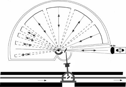
Fig. 15.5. Neutron flight-path diagram: It demonstrates the filter action of the various disks of the chopper cascade. The vertical axis represents the flight-path between the di erent elements of the chopper cascade. CH1 defines the initial timedistribution of the neutron pulse; CHP is the pre-monochromator; CHR is employed for pulse frequency reduction, in order to avoid frame-overlap at the detectors; fi- nally, CH2 selects the “monochromatic” wavelength band for the experiment. The TOF spectra shown schematically on the top of the figure, correspond to a study of the rotational motion of OH− ions [43] with the MTOF spectrometer IN5 at ILL, carried out in 1975 using 4 ˚A neutrons. Each spectrum covers one TOF period Pspec; see text for more details (from [31])
parameters. The most important and unique feature of this type of instrument is the capability of varying the energy resolution continuously over several orders of magnitude (see Sect. 15.2.3). We therefore give here explicitly an expression for ∆( ω). The energy resolution width (HWHM) at the detector [32], i.e., the uncertainty in the experimentally determined energy transferω, is given by
∆( ω) [ eV ] = 647.2(A2 + B2 + C2)1/2/(L12LSDλ3)/2, |
(15.34) |
|||||||
where |
|
|
|
|
|
|
|
(15.35) |
A = 252.78 ∆L λ L12 |
|
|||||||
B = τ |
(L |
+ L |
SD |
λ3/λ3) |
(15.36) |
|||
|
i |
|
2S |
|
0 |
|
|
|
C = τ |
(L |
|
+ L + L λ3 |
/λ3) |
(15.37) |
|||
ii |
12 |
|
2S |
|
SD |
0 |
|
|
∆L is the uncertainty of the length of the neutron flight path, which is mainly due to beam divergence, sample geometry, and detector thickness. The
328 R.E. Lechner et al.
constant coe cients in Eqs. 15.34 and 15.35 are valid, when the quantities L12, L2S , LSD, ∆L are given in [m], λ0 and λ in [˚A], τi and τii in [ s].
It follows from these expressions, that the energy dependent resolution, for given λ0, strongly depends on the scattered neutron wavelength λ, whereas the total intensity, as an integral property of the spectrometer, has no such dependence. Furthermore, high resolution is favored by short pulse widths and by large values of the distances L12 and LSD. If these distances are fixed, and if sample geometry, λ0 and energy transfer have been chosen, then total intensity and resolution-width only depend on the chopper opening times τi and τii. Best instrument performance regarding intensity and resolution is achieved not only by selecting suitable values of the individual pulse widths, τi and τii, but also requires the optimization of their ratio (pulse-width ratio (PWR) optimization [32, 38]). The optimization formula for elastic and quasielastic scattering is shown as an inset in Fig. 15.4.
The continuous variation of the energy resolution over three orders of magnitude is achieved by varying the chopper pulse widths τi and τii (which, e.g., in the case of NEAT is possible by a factor between 1 and 40), and by choosing the incident wavelength (yielding another factor, of up to about 30 for the wavelength range from 4 to 12 ˚A). Applications of this technique using the MTOF spectrometer NEAT at HMI in Berlin, are described in Sects. 16.3.4 and 16.4.3 of Part II, this volume.
15.3.3 XTL–XTL Spectrometers
The energy-transfer regime in the eV range is covered by back scattering (BSC) spectrometry [45–48], which was invented by H. Maier-Leibnitz. BSCspectrometers are XTL–XTL instruments, i.e., they employ single-crystals as monochromators and as analyzers, with Bragg angles close to π/2 in both cases. For a given incident divergence of the beam, ∆Θ, the wave number spread produced by reflection from a crystal is given by di erentiating Eq. 15.31
∆kdiv |
= cot Θ ∆Θ . |
(15.38) |
|
k |
|||
|
|
For typical Bragg angles and ∆kdiv/k ≈ 10−2 rad one achieves an energy resolution in the percent range. However, for Θ approaching π/2, ∆kdiv from Eq. 15.38 goes to zero and we have to include the curvature of sin Θ which leads to a second order contribution,
∆kdiv |
= |
(∆Θ)2 |
for Θ → |
π |
(15.39) |
||
|
|
|
|
. |
|||
k |
8 |
2 |
|||||
This situation is called “backscattering” which means that the incident and the Bragg reflected beam are practically antiparallel. The square relation Eq. 15.39 replaces the linear relation between ∆kdiv and ∆Θ: The intensity is proportional to the incident solid angle (∆Θ)2, and we have (∆Θ)2 ∆kdiv
15 Quasielastic Neutron Scattering: Methods |
329 |
instead of ∆Θ ∆kdiv, which is valid for Bragg angles other than π/2. This means that under these conditions resolution and intensity are decoupled in first order.
Actually, the wavevector spread is larger than ∆kdiv. Only a finite number of lattice planes contribute to the Bragg line, which causes a finite width of G, the so-called Darwin or extinction width [49],
∆kex |
= |
16πNcFG |
, |
(15.40) |
|
k |
|
G2 |
|||
|
|
|
|
||
where FG is the structure factor for the Bragg reflection at Q = G, Nc is the number of lattice cells per unit volume. As an approximation, both contributions can be added such that
∆E0 |
= 2 |
|
(∆Θ)2 |
+ |
16NcFG |
. |
(15.41) |
|
E0 |
8 |
|
G2 |
|||||
For neutrons from an Ni neutron guide and reflection on an ideal silicon waver, one calculates ∆E0 = (0.24+0.08) µeV as incident neutron energy spread. For the resolution in energy transfer, ∆( ω), of a modern BSC-spectrometer, such as the BSC-spectrometer IN16 (Fig. 15.6) at the ILL high-flux reactor [47,48], one obtains values of 0.09, 0.2, and 0.43 µeV (HWHM), depending on the type of monochromator and analyzer crystals used [48]. So far such values have not been reached by any other kind of crystal spectrometer; they can in principle, however, be achieved also by high-resolution TOF–TOF instruments at future spallation sources [31].
The high energy resolution of IN16 is based on a Bragg angle fixed at 90◦; the energy scan is performed by a Doppler drive, moving the monochromator crystal (spherical, perfect Si(111), 450 × 250 mm2; label 6 in Fig. 15.6) with a sinusoidally varying speed vD. The resulting energy shift is [50]
|
δE0 |
= 2 |
vD |
(15.42) |
|
E0 |
v0 |
||||
|
|
|
which yields an energy window of δE0 = ±14 µeV for maximum speed values of vD = ±2.5 ms−1 and λ0 = 6.27 ˚A. The various components of the instrument are arranged as follows: A double-deflector array (1 and 5 in Fig. 15.6) selects the useful wavelength band from the cold-neutron guide. The first deflector (1 in Fig. 15.6), a (broad-band) vertically focusing pyrolythic graphite crystal separates the neutrons to be used from the incident beam and reflects the whole energy-transfer range of about ±14 µeV, covered by the Doppler motion of the monochromator, into a NiTi supermirror guide (2 in Fig. 15.6). The latter focuses these neutrons vertically and horizontally onto the second deflector (5 in Fig. 15.6). A Be-filter and a background chopper (3 and 4, respectively, in Fig. 15.6) are located in a gap in the middle of this guide. The second deflector (label 5 in Fig. 15.6), made of PG(002) crystals with a wide mosaic, is mounted on a chopper wheel with alternating open and reflecting segments. It sends a neutron pulse towards the monochromator (label 6
330 R.E. Lechner et al.
8
7
6
5
9
4
3
2
1
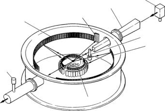
Fig. 15.6. BSC-spectrometer IN16 at the ILL high-flux reactor [47, 48], schematic view: 1 = first graphite deflector crystal; 2 = focusing supermirror guide; 3 = Beryllium-Filter; 4 = background chopper; 5 = stationary graphite-crystal deflector chopper; 6 = Doppler monochromator crystal; 7 = sample; 8 = spherically arranged analyzer crystal array; 9 = multitube detector array. The Bragg angles at the silicon single crystals (i.e., monochromator and analyzer, before and after scattering of the neutrons by the sample) are close to 90◦. Other well-known spectrometers of this type are the BSC-spectrometer at the J¨ulich FRJ-2 reactor, IN10 [46] and IN13 at ILL in Grenoble, France, and HFBS [51] at NIST in Gaithersburg, USA
in Fig. 15.6). The monochromatic backscattered neutron pulse is transmitted through the open segments to the sample. Obviously the system is designed in such a way, that the necessary phase relations between Doppler drive, deflector chopper, and background chopper are observed. To avoid that the scattered neutrons are directly falling onto the detectors (before they have been filtered by the Si analyzers), the incident beam is periodically interrupted by the background chopper, in phase with the Doppler movement. Only when the beam is closed, the consecutively scattered and analyzed neutrons reach the detectors. This ensures that the useful neutrons are reaching the sample, the analyzers, and finally the detectors, while the background that would be caused by neutrons scattered without energy analysis from the sample directly into the detectors, is discriminated. The monochromatic neutrons from the oscillating monochromator crystal, falling onto the sample, being scattered, and finally detected, are individually labelled with the corresponding instantaneous speed
15 Quasielastic Neutron Scattering: Methods |
331 |
of the Doppler drive. The neutrons scattered by the sample are backscattered by spherical shells of Si(111) crystals and thus focussed into a set of 3He detectors. Each detector corresponds to a certain scattering angle or Q-value. When the energy range is too narrow, the reflected neutron energy can be additionally shifted by heating the monochromator, thus increasing the lattice parameter, and/or using monochromators whose lattice parameter is somewhat smaller or bigger than that of the silicon analyzer [52]. In this way, the range of the spectrometer (and also the resolution) can be adapted to the problems.
Sometimes, BSC-spectrometers are used with the Doppler drive at rest, i.e., in the so-called elastic-window scan mode of operation (see [53], [54] and [23] p. 284). In such a measurement one determines the intensity for the spectrometer set at ω = 0, corresponding to the convolution integral [Ss(Q, ω = 0)]meas = (Ss R), where as an example, Ss is the incoherent neutron scattering
function and R is the energy resolution function (see Eq. 15.29). For scattering functions with Gaussian shape in reciprocal space, when they permit a time-independent atomic mean-square displacement to be defined (e.g., for harmonic vibrations), and when the nonelastic scattering contribution to the elastic channel is negligible, the Q-dependence of the scattered intensity at zero energy transfer reads:
Ss(Q, ω = 0) = C exp [− < u2 > Q2], |
(15.43) |
where C is a normalization factor, the exponential is the Debye–Waller factor, and u is the component of the atomic displacement along the vector Q. This expression may also be employed for any spatially restricted isotropic motion, as long as Q is small enough (Gaussian approximation; see Sect. 16.3 in Part II of this chapter, in this volume). It has even been used for non-Gaussian probability density distributions, for instance in the context of the so-called “dynamical transition” [55–59] (see Sect. 16.5.2 in Part II ; see also the article by Lehnert and Weik in this volume). This is justified, as long as one keeps in mind, that in such cases the quantity < u2 > becomes a phenomenological parameter with a less precise meaning than in the harmonic-vibration case. This parameter can be used for the qualitative study of the e ects due to the variation of external variables, such as the temperature.
Let us now consider a case, where the scattering function has an appreciable quasielastic component, with a temperature-dependent width of the same order of magnitude as the energy resolution of the instrument. For instance, for a Lorentzian-shaped spectrum Ss(Q, ω) = (Γ/π)/(Γ 2 + ω2) (see for instance Eqs. 15.7 or 15.25 in Part II of this volume), and assuming a Lorentzian shape for the resolution function as well (approximately valid for the classical BSC spectrometer), with a width (HWHM) ∆( ω), one obtains for the measured
window-scan intensity at zero energy transfer, |
|
|
|
||||
I(Q, ω = 0, T ) = |
1 |
|
|
1 |
. |
(15.44) |
|
π (Γ (Q, T ) + ∆( ω)) |
|||||||
|
|
|
|||||

332 R.E. Lechner et al.
We will now, for the purpose of discussion, assume that in our example a single relaxation process (responsible for the Lorentzian line shape) is active over the whole temperature range considered, and that it shows an Arrhenius type behavior. Then, for su ciently small temperatures, the quasielastic line falls entirely into the energy resolution window. Therefore, it does not cause any measurable quasielastic broadening. Then one gets for the window-scan intensity:
I(Q, ω = 0, T ) = |
1 |
(15.45) |
(π∆( ω)) . |
With increasing temperature, the line width Γ grows, and finally becomes larger than the window ∆( ω); the measured intensity of the window scan then reveals a “stepwise” decrease. Therefore, a simple temperature scan allows to get a qualitative survey of the di usion or relaxation processes in the sample as a function of temperature.
The intensity “step” represents a (purely methodical) transition from nonobservability at low T to observability at high T of the relaxation process. From the shape of this step the relaxation time of the single process can easily be determined. Let us consider this problem for the more complex situation of a localized di usive process, implying an elastic in addition to a quasielastic Lorentzian component. Here the same experimental method can be applied. If the attenuating e ect of (harmonic) vibrational motions is described by a classical Debye–Waller factor, the temperature-dependent window-scan intensity, in logarithmic form, is given by [60]
ln(I) = −CT Q2 + ln(A(Q)/(π∆( ω)) + (1 − A(Q))/[π(2 /τ2S + ∆( ω))]. (15.46)
Here CT is the vibrational mean square displacement (with a temperature coe cient C), A(Q) is the EISF, and τ2S is the relaxation time (for a twosite jump model in our example; see Fig. 15.1 and Table 15.1). It is interesting to note that the observability transition described by Eq. 15.46 can be used not only to yield the relaxation time τ2S, but also for the determination of the EISF, provided that the mechanism does not change in the T -region of the step. For this purpose, the measured low-temperature straight line of ln(I) vs. T is extrapolated to high T and compared with the measured high-temperature line; the latter is obtained, when due to strongly increased line-broadening, the quasielastic contribution to the intensity becomes negligible. A simple division of the intensities yields the EISF according to the equation [60]
|
extrapol |
. |
(15.47) |
ln[A(Q)/(π∆( ω))] = [ln(I)high T ] − ln(I)low T |
|||
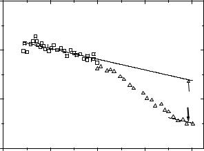
As an example of such a measurement, Fig. 15.7 |
shows the intensity step due |
||
to the e ect of OH-group reorientations in CsOH· H2O [60] appearing in the energy resolution window of the BSC spectrometer IN13.
The elastic-window scan method has been employed in numerous biological experiments, in order to determine the temperature dependence of motional amplitudes (“mean-square displacements”), for instance in the context of the “dynamical transition” (see Sect. 16.5.2 in Part II, this volume).
15 Quasielastic Neutron Scattering: Methods |
333 |
8.5 |
|
|
|
|
|
|
C=3.92 10−4 Å2 T−1 |
|
|
8.0 |
|
|
|
|
ln(I) |
|
|
|
|
7.5 |
EISF=0.69 |
|
|
ln(EISF) |
|
|
|
||
7.0 |
|
|
|
|
0 |
100 |
200 |
300 |
400 |
temperature [K]
Fig. 15.7. Example of an apparent observability transition (as opposed to a true dynamical transition, where due to a structural phase transition a new type of motion appears at a transition temperature or in a transition region, in case of a higher order transition) exhibited experimentally by the elastic intensity I of CsOH · H2O measured as a function of temperature: Logarithmic plot of the elastic-window intensity obtained with IN13 (ILL Grenoble) at Q = 1.89 ˚A−1. The straight lines show the variation of the Debye–Waller factor in the limits of low T and high T , respectively. The logarithm of the EISF is simply the di erence between the values of the two lines at a given temperature [60]
15.3.4 TOF–XTL Spectrometers
Last, but not least, the TOF–XTL technique should be mentioned. This type of hybrid instrument, employs a pulsed polychromatic (“white”) incident beam and single-crystals as analyzing filters. It is well adapted to the time-structure of spallation neutron sources. The energies of the incident neutrons are measured with TOF techniques, while the energy of scattered neutrons is fixed by the analyzers. For high energy resolution the crystals are used in BSC or near-BSC geometry (θ π/2 ), whereas for more moderate resolution θ < π/2 is chosen. Since the quality requirements for the crystals depend on these configurations, and for other practical reasons, dedicated instruments have been built for each case. A typical example with analyzer in near-BSC geometry is represented by the inverted geometry instrument IRIS schematically depicted in Fig. 15.8 [61] at RAL in Chilton. Depending on the type of crystals used, several discrete values of energy resolution in the range from about 1 to 55 eV are achieved. The energy resolution function of such a spectrometer is essentially given by the convolution
15 Quasielastic Neutron Scattering: Methods |
335 |
For IRIS, an example of application is described in Sect. 16.5.1 (see Figs. 16.13 and 16.14 of Part II in this volume).
An example of an inverted-geometry instrument with analyzer scattering configuration significantly deviating from the BSC geometry, is the spectrometer “QENS” at the Intense Pulsed Neutron Source (IPNS) (Argonne, Illinois) [62]. The 22 crystal-analyzer detector-arrays are installed as close as possible to the sample, in order to maximize the analyzed range of solid angle. The crystals are arranged so that they match the “time-focusing-condition” which minimizes the time uncertainty contribution to the resolution. The elastic energy resolution of the spectrometer is around 80 eV. An interesting feature of these spectrometers is the possibility to measure – simultaneously with the quasielastic spectra – the di raction pattern of the sample. This is achieved by scattering from the sample directly into additional detectors, over a very wide wavevector range (up to 30 ˚A−1 in the case of “QENS”), because of the white beam arriving on the sample.
15.4 Instruments for QENS Spectroscopy in (Q, t)-Space
15.4.1 NSE Spectrometers
Di erently from the procedures employed by the QENS techniques discussed in Sect. 15.3, which are based on energy transfer analysis, it is also possible to study scattered neutron intensities by Fourier time analysis. Before discussing neutron spin–echo techniques already well-known for this type of analysis, we briefly mention another method recently proposed [63, 64], which has not yet been widely used. It is based on the measurement of the elastically scattered neutron intensity as a function of observation time. If the latter is properly related to the Fourier time, a direct determination of the intermediate scattering function is achieved, without the detour via Fourier transformation. This method has been proposed as an alternative to energy transfer analysis in the use of TOF–TOF techniques capable of continuous tuning of the energy resolution, a feature so far not available on spectrometers employing crystals as monochromators and/or analyzers.
Let us now turn to the NSE method. It was introduced in 1972 by Mezei [65]. For detailed information on this technique, see [66]. NSE measures the sample dynamics in the time domain, via the determination of the intermediate scattering functions (see Eqs. 15.8 and 15.9). These functions are measured over a range of several orders of magnitude of Fourier time, up to values as large as 10−7 s. The drastic reduction of intensity necessarily arising, when in measurements with energy-analyzing QENS techniques the energy resolution is increased by reducing the incident and/or scattered neutron energy band widths, is circumvented here. This property of the NSE method is a consequence of the fact, that the energy transfer occurring in