

Neutron Scattering in Biology - Fitter Gutberlet and Katsaras
.pdf234 C.F. Majkrzak et al.
reflection from such structures tends to be concentrated at higher Q-values than for single-layer thin films, the Born approximation can be particularly valuable in analyzing reflection from them. For a periodic multilayer structure (assuming ideally flat, parallel layers of uniform density and thickness), the reflection amplitude in the BA is given by ( [28], for example)
|
4π |
|
sin(M QD/2) |
ei(M −1)DQ/2 |
0 |
D |
|
|
rMLBA (Q) = |
ρ(z)eiQz dz , |
(12.13) |
||||||
|
|
|||||||
iQ |
sin(QD/2) |
for M repeats of a unit film (e.g., the bilayer) of thickness D. The integral over ρ(z) is limited to the unit film. The e ect of the M repeats appears only in the prefactor, where (using L’Hospital’s rule) the ratio of sine functions in brackets acts as a concentrator of reflection about the Nyquist lattice points, Q = Qm, as M increases, where Qm = 2πm/D for integer m. Thus, for M large (but not so large as to invalidate the BA), rMLBA (Q) is strongly peaked on the Nyquist points, in the manner of Bragg peaks in crystallography. Figure 12.5 compares the reflectivities, calculated with the exact and kinematic formulas, for M = 50 bilayers having the SLD profile of Fig. 12.4 (and assuming no substrate). Note how the reflected intensity of the multilayer is localized about the Nyquist lattice, in contrast to being more uniformly distributed over the entire Q-range, as evident in Fig. 12.4. Clearly the kinematic theory can give a good account of multilayer reflection.
Now the SLD profile of Fig. 12.4 is centrosymmetric along the z-axis and can, consequently, be represented by a Fourier cosine series [30]
Reflectivity
∞
ρ(z) = A0 + 2 Am cos (Qmz) , |
(12.14) |
m=1 |
|
0.01
0.0001
1e-06
1e-08
1e-10
1e-12
1e-14
0.2 |
0.4 |
0.6 |
0.8 |
1 |
1.2 |
Q (Å−1)
Fig. 12.5. Comparison of the reflectivities, calculated according to the exact and kinematic formulas, for M = 50 bilayers having the SLD profile of Fig. 12.4 (assuming no substrate)
12 Membranes in Biology by Neutron Reflectometry |
235 |
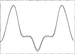
where the Am are real numbers. From the reflectivity curve plotted in Fig. 12.5 (corresponding to the bilayer of Fig. 12.4, with M = 50), the peaks up to the 10th order, inclusive, were used to determine the Fourier series of Eq. 12.14, truncated at m = 10. The resulting ρ(z) is plotted in Fig. 12.6, along with the original SLD profile of Fig. 12.4 for comparison. The agreement displayed in Fig. 12.6 is qualitatively good. But even ten perfectly “measured” orders do not provide all the detail in the veridical ρ(z).
12.2.4 Scale of Spatial Resolution
In assessing the value of SLD profiles inferred from reflection measurements, we must know how much spatial detail is meaningful to expect from the analysis; i.e., we can ask, what is the scale of spatial resolution – let us quantify this as a length l – of the resulting ρ(z)?
Let us say that we have perfect knowledge of the reflection amplitude r(Q) up to a maximum value of Q = Qmax. (The experimental factors determining Qmax will be discussed in a later section.) The dominant factor limiting the spatial resolution of ρ(z) inferred from this knowledge is the value of Qmax, according to = π/Qmax [11,12]. For our purposes, this holds that the number of spatial degrees of freedom N in ρ(z) for a film of thickness L, when r(Q) is known for |Q| ≤ Qmax is given by (the integer part of) N = QmaxL/π, referred to variously as the Nyquist or the Slepian number. Associating the corresponding scale of spatial resolution with = L/N , one has = π/Qmax directly. In addition [12], also emerges explicitly from wavelet representations of ρ(z), where is identified with the scale length of its most rapidly varying “detail,” and N is the number of wavelets needed to fully describe ρ(z) on this length scale. Indeed [11], as a special case, if we model ρ(z) by N bins of uniform SLD
|
1.5e-06 |
|
|
1e-06 |
|
) |
|
|
2− |
|
|
(Å |
5e-07 |
|
r |
|
|
|
|
|
|
0 |
|
|
−5e-07 0 |
5 10 15 20 25 30 35 40 45 50 |
|
|
z (Å) |
Fig. 12.6. SLD profile of Fig. 12.4 (dashed curve) compared to that obtained by the Fourier series analysis of the reflectivity curve (exact result) in Fig. 12.5 described in the text
236 C.F. Majkrzak et al.
and equal widths , as in ρpwc(z) of Eq. 12.3, then rBA(Q) in Eq. 12.12 is exactly invertible for ρpwc(z) over the Q-range, |Q| ≤ Qmax, where Qmax = π/ .
Now in general [12], let r(Q) be perfectly known for |Q| ≤ Qmax, and call this conditional knowledge the function r(Q|Qmax). Then the inversion of r(Q|Qmax) by a fixed procedure – namely the one we would use for Qmax = ∞, but setting r(Q|Qmax) = 0 for Q > Qmax – determines a distorted or “smeared” version of the veridical ρ(z), say ρ(z|Qmax), which effectively parameterizes ρ(z) on the spatial scale . The maximum Q of the measurement thus inherently limits the spatial resolution of ρ(z) that can be reliably determined; the larger the value of Qmax, the smaller the scale of detail we can know reliably.
What if our knowledge is limited to the reflectivity |r(Q|Qmax)|2? If we consider the Born approximation, Eq. 12.12, as an adequate basis for analysis, then we may appeal to the well-known result that the Fourier transform of Q2|rBA(Q)|2 directly determines the auto-correlation function
∞ |
|
γ(z) = −∞ ρ(z − z )ρ(z ) dz , |
(12.15) |
which describes the smearing of ρ(z) by itself. This implies that for given Qmax, if ρ(z|Qmax) is resolved to scale , then γ(z|Qmax) is resolved to scale 2 . More carefully, if ρ(z) is supported on an interval of length L, then γ(z) has support of length 2L. Thus applying the same number of spatial degrees of freedom to ρ(z|Qmax) and to γ(z|Qmax) leads to a scale of resolution 2 = 2π/Qmax for the latter. The loss of phase information thus leads to a loss of spatial resolution for finite Qmax.
12.3 Basic Experimental Methods
Neutron reflection can be done at both pulsed and continuous neutron sources. The only essential di erences between them in regard to instrumental technique involve the means by which neutrons of di erent wavelengths are utilized and identified. With pulsed sources, the broad spectrum of wavelengths present in each pulse can be used because, for elastic scattering, the wavelength distribution of the beam can be determined by time-of-flight measurement. For continuous sources, a relatively narrow band of wavelengths, as defined by a crystal monochromator, is typically employed. The discussions to follow assume a continuous beam; for the most part, however, the experimental methodology described is applicable to pulsed beam reflectometers as well.
Another relatively general classification of neutron reflectometers can be made. For studying interfaces between solid and another solid, fluid, or gas, a sample can be oriented with its reflecting surface(s) vertical (and with the scattering plane, as defined by nominal incident and reflected wavevectors, horizontal). On the other hand, practical study of gas–fluid interfaces needs
12 Membranes in Biology by Neutron Reflectometry |
237 |
the liquid to be horizontal. The primary di erence between these two types of reflectometers involves the mechanisms employed to direct the incident beam onto the sample and subsequently detect the reflected beam. For the sake of conceptual simplicity, we will assume the reflecting surface(s) of the sample to be vertical so that the nominal direction of the incident beam remains fixed relative to its source. Again, this choice does not limit, in any essential way, the relevance of the discussion to the one configuration.
12.3.1 Instrumental Configuration
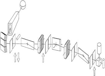
Figure 12.7 is a schematic diagram of a typical neutron reflectometer, which is representative of the NG-1 reflectometer at the NIST Center for Neutron Research. The polarizing and spin flipping devices shown can be ignored for the present discussion, but are essential for magnetization depth profile measurements performed with polarized beams [32]. Within the core of the reactor, neutrons are produced by nuclear fission. The relatively high energies of these neutrons are subsequently moderated by collisions with heavy water at room temperature, resulting in a characteristic distribution of wavelengths with a peak in elastically reflected intensity (for Q = 0.1 ˚A−1, and ∆Q/Q = 0.05) occurring at a wavelength about 1.5 ˚A. The energy distribution is further moderated by the liquid hydrogen “cold source,” shown schematically in Fig. 12.7, shifting the peak in elastically reflected intensity to approximately 5 ˚A. The beam of cold neutrons is transported through an evacuated rectangular guide, the smooth, flat interior walls of
|
Liqiud hydrogen cold source |
|
|
NG-1 Reflecting |
|
|
|
Guide tube |
|
|
|
|
Incident beam |
|
|
|
intensity monitor |
|
|
|
Sample |
Higher-order |
|
|
|
||
|
Fe/Si supermirror |
wavelength |
|
|
polarization |
be filter |
|
|
analyser |
|
|
|
Fe/Si supermirror |
|
|
Vertically focusing |
polarizer |
|
|
|
|
||
PG(002) |
Neutron |
|
|
triple crystal |
Detector |
||
spin-flipper |
|||
monochromator |
|
|
|
|
Vertical slit |
|
Fig. 12.7. Schematic of a typical neutron reflectometer (representative of the NG-1 polarized beam reflectometer at the NIST Center for Neutron Research; the polarizing and spin flipping devices are used in the determination of the vector magnetization depth profile in magnetic films and can be ignored for this presentation)
238 C.F. Majkrzak et al.
which are coated with a Ni film which gives a relatively large critical angle for total external or mirror reflection of about 0.1 deg ˚A−1 of incident wavelength.
This beam then impinges upon a pyrolytic graphite monochromating crystal array which Bragg reflects a vertically focussed beam onto the sample. The (002) atomic planes of the graphite crystal reflect a beam with a nominal wavelength λ = 4.75 ˚A for the chosen 90o scattering angle 2θM(λ = 2d sin θM), where d is the (002) atomic plane spacing, approximately 3.354 ˚A, and θM is the glancing angle of incidence measured from the crystal surface. The pyrolytic graphite consists of microcrystallites, which are essentially perfect single crystals of hexagonally arrayed carbon atoms, having dimensions of hundreds to thousands of ˚Angstroms, both along the (002) direction and perpendicular to it.
The beam reflected onto the sample by the monochromating crystal has a wavelength distribution determined mainly by the angular distribution of neutrons within the guide, the FWHM of the angular distribution of the graphite crystal’s mosaic blocks, the interplanar spacing of the (002) graphite atomic planes, and the horizontal angular collimation of the beam (defined by the pair of vertical slits preceding the sample, as shown in Fig. 12.7.) A typical horizontal angular divergence is between 1 min and 10 min of arc, and because this is relatively small compared with that in the guide and the crystal mosaic angular spread, the wavelength resolution, ∆λ/λ, principally depends on the latter two fixed quantities and is about 1 %.
As pictured in Fig. 12.7, each finger of a vertically focusing monochromator array is a stack of several graphite crystals, slightly inclined relative to one another, so as to create a broader (but e ectively anisotropic) mosaic, thereby widening the wavelength band (to increase the intensity within the limits allowed by a given Q-resolution). At the NCNR NG-1 reflectometer, the 15 cm beam height in the guide is focused down to about 3 cm at the sample position so that the vertical angular divergence is approximately 2.5o. For specular reflectivity measurements, this relatively relaxed vertical angular divergence has a negligible e ect on the Q-resolution.
Downstream of the sample position is a second pair of slits before the detector which are primarily used to suppress incoherent scattering background. For specular reflectivity measurements, the wavelength distribution and angular divergence of the incident beam, in conjunction with the glancing angle of incidence that the beam makes with the surface of a flat sample, determine a nominal value of Q and its associated resolution width. In addition, the slit just before the detector is needed to properly shape the instrumental resolution function in performing non-specular scattering scans perpendicular to the specular direction. In the latter case, the slit before the detector is significantly narrowed as the sample angle is rotated with the detector at a fixed scattering angle (this results in a trajectory in reciprocal space that is nearly orthogonal to the specular direction for su ciently small angles).
12 Membranes in Biology by Neutron Reflectometry |
239 |
For a sample that is distorted enough from perfect flatness, slits following the sample may block contributions to the reflected intensity from certain distorted regions of the sample surface from reaching the detector, thereby e ectively improving the Q-resolution for specular reflection.
12.3.2 Instrumental Resolution
and the Intrinsic Coherence Lengths of the Neutron
The theory of neutron reflection discussed in Section 12.2 assumed that each neutron in a beam of noninteracting, independent particles could be described by a single plane wave of infinite spatial extent. Generally, a neutron is more accurately described as a superposition of component plane waves, commonly known as a wave packet [13]. The wave packet description follows from localization of the neutron in space and imparts characteristic coherence lengths, both parallel and perpendicular to the direction of propagation defined by a nominal neutron wavevector k. These lengths – a measure of the combined uncertainties in position and momentum that must be associated with an individual neutron – determine the e ective volume of the scattering medium with which the neutron wave packets coherently interact, and, consequently, they are important to interpret specular reflectivity data. However, because the neutrons constituting the incident beam originate from di erent, uncorrelated points within the source, there is an additional component of uncertainty in a distribution of nominal neutron wavevectors. This incoherent component can dominate the coherent, wave-packet-spread component, ultimately leading to the familiar “instrumental resolution” distribution in Q. In-depth, quantitative treatments of neutron coherence and instrumental resolution are given in several places [33–38]. Nonetheless, it is worthwhile here to consider these points further, at least qualitatively.
Incoherent vs. Coherent E ects
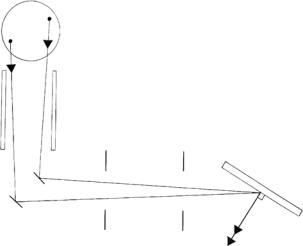
Figure 12.8 shows a liquid hydrogen moderator which acts as an incoherent source of neutrons for a specular reflectivity experiment to be performed downstream in a geometrically well-defined beam. Each of two neutrons, “A” and “B”, radiates from a separate region of the liquid hydrogen cold source, as a result of an incoherent scattering event involving a single hydrogen nucleus. In general, all the coherent interactions of either neutron with objects along its path to the sample – e.g., the guide walls, a particular monochromator microcrystallite, and the pair of rectangular apertures preceding the sample
– contribute to redefining the size and shape of the wave packet representing that neutron when it eventually encounters the sample. Nonetheless, let us assume that neutrons A and B are represented by wave packets of the same size and shape. Each neutron wave packet then possesses the same characteristic coherence lengths related to the uncertainties in position (∆x, ∆y, ∆z)
240 C.F. Majkrzak et al.
EXTENDED LIQUID
HYDROGEN COLD SOURCE
B
A
GUIDE TUBE
CRYSTAL
MONOCHROMATORS
PAIR OF
APERTURES
FLAT |
SAMPLE |
|
|
Q |
|
A |
|
Q |
|
B |
|
Fig. 12.8. Schematic representation of two independent, noninteracting neutrons, “A” and “B”, emanating from di erent places in the cold source and passing through common instrumental optical elements en route to the sample. The size and shape of the wave packet describing neutron A is similar to that of B, but each packet has a di erent nominal wavevector direction. See the discussion in the text regarding coherent vs. incoherent components of the e ective instrumental resolution
and wavevector (∆kx, ∆ky , ∆kz ) of the neutron, that, as mentioned above, define a volume over which the neutron interacts with the sample. Any size and shape wave packet is an appropriately weighted superposition of plane waves [13]. The two neutrons travel in di erent directions, defined by their nominal wavevectors, so that each neutron is Bragg reflected from a separate monochromator crystal segment (but through the same pair of apertures) onto the sample. The latter fact means that the values of the normal component of the incident wavevector k0z = Q/2 for the two neutrons di er from one another.
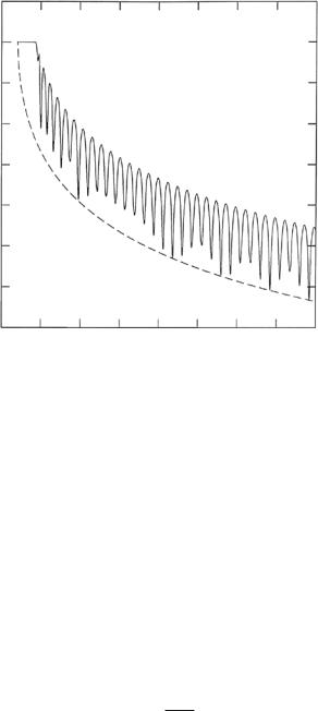
For specular reflection, we need only consider the z-axis normal to the plane of the film. In practice, at a continuous source, specular reflection measurements are performed with neutrons having nearly the same nominal k0 incident at di erent glancing angles θ, so that the resulting range of k0z = k0 sin θ values are obtained by changing the angle of incidence. Then, the relevant longitudinal coherence length e ectively is the projection of the neutron wave packet coherence length along z. (See [39] for the case of normal incidence with ultra-cold neutrons.) The reflectivity, |r|2, which results for a single plane wave incident on a perfectly flat and homogeneous Ni film 1,000 ˚A thick is plotted in Fig. 12.9. As is well-known, the oscillations evident in Fig. 12.9, the so-called “Kiessig fringes”, are produced by interference
12 Membranes in Biology by Neutron Reflectometry |
241 |
Reflectivity
10
Log
1
−1
−3
−5
−7 |
|
|
|
|
0.00 |
0.05 |
0.10 |
0.15 |
0.20 |
|
|
Q (Å−1) |
|
|
Fig. 12.9. Specular neutron reflectivity for a free-standing Ni film, 1,000 ˚A thick. The oscillations are a result of the interference which occurs in the simultaneous scattering of the wave from front and back surfaces of the film, as discussed in the text. The period of the oscillations is approximately 2π/L
between parts of the wave that are scattered from front and back film surfaces; the period of the oscillations is approximately 2π/L. Such interference requires that the incident plane wave interact with both interfaces “coherently,” i.e., simultaneously.
For a one-dimensional incident wave packet with a finite characteristic coherence length along the z-axis Eq. 12.1 must be solved. We can describe the incident wave function as a wave packet ψWP(z)coh consisting of a superposition of plane waves, each component having a well-defined value of kz , viz.,
∞
ψWPcoh (z) = |
φ(kz |k0z )eikz z dkz , |
(12.16) |
|
−∞ |
|
where the normalized weighting φ(kz |k0z ) might, for instance, be represented by a Gaussian distribution centered on the nominal k0z , viz.,
|
|
|
|
|
−4 ln 2 |
(kz k0z )2 |
|
|
|
2 |
|
ln 2 |
|
|
|
||
|
2 |
− |
|
|
||||
φ(kz ) = |
|
|
e Γcoh |
, |
(12.17) |
|||
Γcoh |
π |
|||||||
where Γcoh is the FWHM of the distribution. For such a Gaussian wave packet, the relationship between uncertainties ∆kz and ∆z of wavevector and position,

242 C.F. Majkrzak et al.
respectively, along z is given by the Heisenberg uncertainty relation
∆z∆kz = |
1 |
(12.18) |
2 . |
Although we will not explicitly solve the wave equation for the case of an incident wave packet here, let us call the result of that calculation for the reflection amplitude rWPcoh (k0z ), where k0z denotes the nominal kz for the wave packet. To a first approximation, rWPcoh is a superposition of “components” r(kz ) with the same weighting φ(kz |k0z ) as in Eq. 12.16. The resulting specular reflectivity for the case where the incident neutron is described as a wave packet with a coherence length L << L along z does not display the pronounced Kiessig fringes appearing in Fig. 12.9 because the degree to which the neutron can coherently interact with front and back surfaces is significantly diminished.
Let us now consider a collection of neutrons which constitute an incident beam. Let us assume that every neutron in the beam is described by the same one-dimensional wave packet and coherence length, but that there now exists a distribution of di erent nominal wavevector magnitudes, k0z , distinct from the distribution of kz about a given k0z in a wave packet. We can, for convenience, choose this distribution also to be Gaussian. However, the distribution of k0z describes an incoherent association of our “test” neutrons A and B, in the sense that each neutron in the beam reflects from the film independently. Thus, the measured reflectivity RM(QM), at nominal Q = QM, for an incident beam of such neutrons is the average over Q = 2k0z of the
wave packet reflectivities |rWPcoh (Q)|2; viz., |
|
|
|
|
||||||
|
2 |
|
|
|
|
∞ |
|
|
QM)2 |
|
|
|
ln 2 |
4 ln2 2 (Q |
|
|
|||||
RM(QM) = |
|
|
|
|
−∞ |rWPcoh (Q/2)|2e− |
Γinc |
− |
dQ , |
(12.19) |
|
Γinc |
|
π |
||||||||
where Γinc is the FWHM of the Q-distribution. The convolution in Eq. 12.19 is the “instrumental resolution” commonly employed – but usually with rWPcoh replaced by r for the ideal case of an incident plane wave – and also contributes to smearing the fringes in Fig. 12.9. Thus, instrumental resolution should be as tight as reasonably possible, especially where eventual knowledge of rWPcoh is the goal of the measurement.
Thus, the source of the neutrons and their interactions with instrumental components, which combine to define the size, shape and direction of each neutron wave packet, determine both coherent and incoherent distributions of possible wavevector components in the measurements. The coherent contribution characterizes the wave packets describing individual neutrons, our A or B, while the incoherent contribution emanates from the pathways taken by di erent neutrons, A and B. For example, di raction by a su ciently narrow slit aperture may significantly distort the nominal neutron plane wave, leading to a coherent distribution of wavevectors (common to A and B), while the mosaic structure of the monochromator induces an incoherent spread of wavevectors incident on the sample, distinguishing A from B.
12 Membranes in Biology by Neutron Reflectometry |
243 |
12.3.3 In-plane Averaging
In-plane structure causes non-specular reflection, as previously mentioned, but even when this is weak enough to be ignored, the observed specular reflection will be influenced by lateral variations of the depth profile. The common assumption is that the laterally averaged scattering length density produces the specular “component” of reflection. That is, if the SLD profile is described everywhere in the film by ρ(x, y, z), then the reflection amplitude r(Q) is caused by its lateral average ρ(z) = ρ(x, y, z) xy , as introduced in Eq. 12.2 and the related discussion. This can be true, however, only to the extent that the neutron beam is laterally coherent over the surface of the film, so that such an average is meaningful.
In three dimensions, we can ascribe two coherence lengths to the incident neutron wave packet: a longitudinal coherence length cohz , which is the coherence length we had in mind in discussing the immediate implications of Eq. 12.18 in terms of film thickness; and a lateral or in-plane coherence lengthcohxy , which limits the size of the surface the incident wave packet “coherently sees.” Note that the coherence lengths discussed here are the projections of the neutron wave packet coherence lengths, parallel and perpendicular to its nominal wavevector, projected onto the coordinate axes of the sample.
Now in Eq. 12.19 we implicitly assumed that the film was laterally homoge-
neous. More generally, however, the reflectivity |
|
rcoh |
|
|
|
|
|
|
|
|
xy |
||
|
|
2 appearing in the “inco- |
|||||||||||
|
|
WP |
|
|
|
|
|
|
|
|
|
||
herent” convolution integral must be replaced by a |
lateral average |
r |
coh |
2 |
. |
||||||||
|
|
||||||||||||
|
|
|
|
|
|
WP |
a film |
||||||
For example, a sample characterized by partial coverage might |
comprise |
||||||||||||
|
|
|
|
|
|
|
|||||||
composed of two (fully and partially covered) components and a corresponding scale of inhomogeneity xy equal to the larger of the dimensions associated with the fully and partially covered regions. In cases where cohxy xy , the film appears to the neutron beam as homogeneous, and the specular reflectivity is caused by the corresponding lateral average, ρ(x, y, z) xy , as in Eq. 12.2. However, when cohxy xy , the film appears, instead, as a collection of several types of films, each of which reflects the neutrons according to their “local” ρ(z). Then the measured reflectivity is an areally weighted average of reflectivities from several di erent films. That is,
|
|
|
|
|
|
|
rcoh |
|
2 |
|
for coh >> xy , |
|
|||
|
coh |
|
2 |
|
|
|
|
|
|||||||
|
|
|
|
|
|
|
|
|
|
||||||
|
rWP |
|
|
|
|
j |
wj |
|
rcoh |
|
2 for xycoh << xy , |
(12.20) |
|||
|
|
|
|
|
|
|
|
|
|
WP,j |
|
|
|
||
where wj is the weighting for the jth type of in-plane component. In the second case, unlike the first, there is no single physically defined ρ(z), so any attempt to analyze the reflectivity in terms of one such SLD profile must fail, unless wJ ≈ 1 for some j = J.
Thus we must ask, how do we know which case of Eq. 12.20 is the correct one for a given experiment? In some cases a visual inspection of the sample may su ce to say; if we can literally see, i.e., with visible light, evidence for