Neutron Scattering in Biology - Fitter Gutberlet and Katsaras

where l is the length of the flight path in the field, and v is the neutron velocity. Typically, 5 ˚A neutrons submitted to a field of 10 G will perform around 37 turns per meter, and when the field is increased to 0.5 T (5000 G) this number can be increased up to 18500.

When the direction of the magnetic field changes, two extreme cases can be considered. Let us, for the sake of simplicity, assume that the neutron spin is initially collinear with the field: (i) Slow (or “adiabatic”) change of the magnetic field: A change of the field direction, encountered by the neutron on its way along the flight path, is experienced as a rotation of the field in the coordinate frame of the flying neutron. This may be represented by an angular frequency ωF of rotation, which depends not only on the spatial variation of the field in the laboratory coordinate frame, but also on the neutron velocity. The spin follows adiabatically the change of the field when ωF ωL: If it was initially collinear with the magnetic field, it will rotate with the latter, i.e., the spin direction is following the field. (ii) Sudden (or “non-adiabatic”) change of the field: this is the limit opposite to the adiabatic change, i.e., ωF ωL; in this case the field variation is so fast that the spin direction can not follow. Such changes are used to initiate the spin precession. This will be explained below.

The Neutron Spin-Echo Principle

The general principle of the neutron spin–echo spectrometer is presented in Fig. 15.9. A neutron of wavelength λ0 moving in direction Z arrives at t = 0 in Z0, with its spin in the |+ state with respect to the Z direction. A π/2 flipper “suddenly” puts the spin state perpendicular to the direction of the field (the description of these flippers is omitted in the context of this book, but the interested reader is referred to [71]). This action initiates a precessional motion in the counter-clockwise sense (the gyromagnetic ratio γ of the neutron is negative).

Let us now assume a beam of polarized neutrons moving perfectly parallel in Z direction (assuming zero beam divergence), with a wavelength distribution f (λ0), the maximum of the distribution being located at λ0. We now want to calculate, what will be the precession angle distribution at ZA, if the field path integrals are equal in the two arms. From Z=0 to the sample position ZS, i.e., in the first arm of the spectrometer, the spin of a neutron of wavelength λ0 will accumulate a total precession angle of

338 R.E. Lechner et al.

Beam polarisation

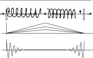
Fig. 15.9. Principle of the neutron spin–echo spectrometer: A neutron of wavelength λ0 moving in direction Z arrives at t = 0 in Z0, with its spin in the |+ state with respect to the Z direction. Two coils create high magnetic fields of equal strength, but in opposite directions, B1 and B2, before and after the sample (upper part). A π/2 flipper “suddenly” puts the spin state of the arriving neutron perpendicular to the direction of the field. This initiates a precessional motion of the neutron spin in the counter-clockwise sense, while this particle is flying along Z. The spin precession stops after a second π/2 spin flipper placed after the end of the second coil. The accumulated spin phases Φi are proportional to the time, wavelength, and distances (central part). The beam polarization P ≈ cos(Φi ) is presented in the lower part of the figure. If the sample is a purely elastic scatterer, the neutron wavelength λ0 is not changed by the scattering process. Because of the two magnetic fields with equal strength but opposite signs, in the case of elastic scattering, the total phase angle accumulated by the neutron spin precession during the flight from Z0 to ZA, will be Φ(λ0) = 0. The general case of nonelastic scattering is explained in the text

where

The analogous quantities can be calculated for the second arm: Let us assume that the sample is a purely elastic scatterer and thus the neutron wavelength λ0 is not changed by the scattering process. From ZS to ZA the neutron is submitted to a magnetic field in direction opposite to the field

before the sample. Then the accumulated precession angle will be

which is the number of (negative) spin turns between ZS and ZA. For any

Finally, we obtain for the total phase angle accumulated by the neutron spin precession of any neutron in the distribution:

It is easy to realize that at the “echo-point”, where the field path integrals in the first and in the second arm of the spectrometer are equal, the total phase angle accumulated by the neutron spin precession will be Φ(λ0) = 0, and this is true for any neutron velocity; i.e., this result is independent of λ0.

Transmission of Polarizers and Analyzers

Polarizer and analyzer are key elements of the spectrometer. The polarizer is used to prepare a polarized beam (i.e., it selects neutrons with only one of the two quantized neutron spin states). For long-wavelength neutrons (λ > 3 ˚A), as are generally used in NSE experiments (at least for quasielastic measurements), most of the polarizers employ the principle of magnetic reflection or transmission of supermirrors. For shorter wavelengths, Haeussler-like crystals are used. A potentially very interesting technique for spin analysis is the use of a 3He polarizer and/or analyzer. For the spin–echo technique a 3He polarizing filter unit would have the very interesting property of being simultaneously usable over a wide angular range and independently of the neutron wavelength. At the time of writing the beam polarization achieved with 3He is however, not yet good enough for spin–echo experiments.

340 R.E. Lechner et al.

The polarizer transmits only neutrons with one of the spin components. The exact fraction of the neutron beam transmitted is not relevant for the principle of the technique, but it should be maximized for the purpose of obtaining good statistical accuracy of the measurements. The number of incident neutrons is usually monitored just before the sample position. For our present purpose, the interesting problems will be: (i) To compute the probability of transmission through the analyzer for a neutron whose spin angle with the static field BA inside the analyzer is given by θ. (ii) To determine the beam polarization of a neutron population whose spin angles are given by the normalized distribution F (θ).

These problems require a quantum-mechanical calculation. The spin-state wave function for the neutron spin precessing in the field BA is

˜

where Φ and θ are the spherical coordinates defining the orientation of the spin with respect to the analyzer field. Each neutron spin will have the probabilities p|+ = cos2 θ2 and p|− = sin2 θ2 , to be either in the |+ or in the |− state, respectively.

The solution of problem 1 is that only |+ neutrons will be transmitted, the probability of transmission being given by p|+ = cos2 θ2 . Thus for a neutron flux N incident on an idealized analyzer (i.e., with no absorption losses), with the normalized spin-precession phase-angle distribution F (θ), the flux of neutrons transmitted by the analyzer will be

Using a well-known trigonometric relation for the square of the cosine, we can compute the transmission of the analyzer

It is straightforward to show that cos(θ) corresponds to the polarization of the transmitted beam,

Getting a Spin-Echo, as a Measure of the Polarization

We now return to Eq. 15.58, because we want to compute the polarization of the scattered beam. We will treat the problem for two di erent cases: (i) The

wavelength of neutrons is not changed by the scattering process. (ii) For a quasielastic distribution of energy exchange between the sample and the neutron beam.

First, assuming a purely elastic scatterer, Φ(λ0) does not depend on the sample, but simply on the incident wavelength distribution f (λ0), which is assumed to be Gaussian. The final beam polarization can then be computed as,

where α was defined by Eq. 15.59, and σ is the standard deviation of the wavelength distribution. The above integral has a simple analytical solution, if the integration is performed from −∞ to +∞, which is possible, because the assumed (in good approximation) Gaussian shape of the distribution to be integrated is practically zero for negative (unphysical) values of the wavelength. The integral yields for the beam polarization

The variation of the beam polarization in the neighborhood of the echo point is shown in Fig. 15.10. It presents a full echo scan around the spin–echo max-

small additional solenoid coil. This variation can be computed. Writing for the field path integral of the solenoid,

˜

B dl = µ0N i , (15.68)

where N is the number of turns of the solenoid wire per unit of length, we get the function (continuous line) plotted together with the measured data points of the full echo scan in Fig. 15.10

where l is the coil length, m the neutron mass, h the Planck’s constant, and µ0 is the permeability of free space. Pe and ie, respectively, are the scattered neutron beam polarization and the current of the NSE tuning coil, at the echo

342 R.E. Lechner et al.

current i[A] in the NSE “tuning” coil

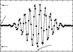
Fig. 15.10. Full echo (asymmetric current scan) measured (full squares) with the spectrometer MUSES [74] at the point ZA, (see Fig. 15.9). The continuous line is the fit of Eq. 15.69 to the measured data points. Pe and ie, respectively, are the scattered

count unit, scattered by the sample towards the analyzer (see text). The maximum and minimum numbers of neutrons that are transmitted by the analyzer, when the current i is varied, N (1 + Pe)/2 and N (1 − Pe)/2, are also indicated. N/2 is the number of neutron counts, when – outside of the spin–echo region – the beam is completely depolarized

The maximum and minimum numbers of neutrons that are transmitted by the analyzer, when the current i is varied, N (1 + Pe)/2 and N (1 − Pe)/2, are indicated by horizontal arrows. N/2 is the number of neutron counts, when – outside of the spin–echo region – the beam is completely depolarized.

Measuring Quasielastic Neutron Scattering

We now assume the scattering process to be quasielastic. The energy exchanged between the neutron and the sample during the scattering process is

This will induce a change δλ of the neutron wavelength, so that for incident neutrons with wavelength λ0 the scattered neutron wavelength is λ = λ0 + δλ. The polarization of the scattered beam can be expressed as follows:

Here, p(λ0, δλ) is the probability that a neutron scattering process with incident wavelength λ0 and with a change in neutron wavelength δλ occurs; note that the maximum possible negative value of δλ is equal to λ0. The function p(λ0, δλ), when transformed from the δλ-transfer to the energy-transfer axis, turns into nothing else but the scattering function S(Q, ω). Φ(λ0, δλ) is the total precession angle. Note also, that writing Eq. 15.72 we have assumed a perfect spectrometer: The incident beam is perfectly polarized, all the neutrons are transmitted through the spectrometer (whatever the wavelength) and with no beam depolarization. We will come back to this assumption, when discussing the di erent spectral windows and resolutions of quasielastic spectrometers. It is important to realize that the total precession angle Φ(λ0, δλ) represents the energy transfer ω which corresponds to the change δλ in neutron wavelength, caused by the scattering process

At the echo point (for QENS experiments, the field path integrals are identical in the first and the second arm) α = 0 and hence

For quasielastic scattering, it is assumed that the energy gained or lost by the neutrons remains much smaller than the initial energy of the neutron, i.e., δλ/λ0 1, hence

0−∞

Note that the second integral in Eq. 15.77 is the real part of the Fouriertransform of the dynamic structure factor S(Q, ω). The spin–echo time τNSE approximates the Fourier time t, and it is important to note that it is

344 R.E. Lechner et al.

proportional to the third power of the wavelength (see also Sect. 15.4.3). Thus, it is now evident that

The ≈ symbol stands for the fact that S(Q, ω) is only approximately a symmetric function in ω, and that the integration over the wavelength distribution I(λ0) in Eq. 15.77 has a certain smearing or broadening e ect on I(Q, t).

The reason, why NSE spectroscopy measures sample dynamics in the time domain, is that the analyzer transforms a quantity proportional to the time, Φ(λ0), into a cosine: cos(Φ(λ0)); the summation over all the scattered intensity ( S(Q, ω)) weighted by this cosine function, Fourier-transforms the dynamic structure factor. One should nevertheless keep in mind, that only the real part of the FT is measured, and thus P I(Q, t) only, if S(Q, ω) is an (almost) even function. This is however, usually the case for NSE experiments, because they probe the very low-frequency part of the dynamic structure factor, where the spectral asymmetry due to the detailed balance factor can be neglected and S(Q, ω) is to a good approximation an even function, as long as the temperature is not too low. For an application of this technique, see Sect. 16.3.2 in Part II of this volume.

15.4.2 Neutron Resonance Spin-Echo Spectrometry

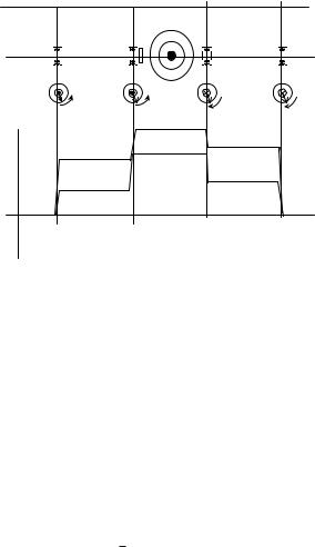
In resonance spin–echo spectrometry [75,76], the two high magnetic-field precession coils are substituted by four radio-frequency coils, two in the first arm and two in the second (see Fig. 15.11). The field geometry in the coils is as follows: a static high field B0, e.g., oriented vertically, and perpendicular to it a radio-frequency field B1(t) rotating in the horizontal plane.

The resonance condition is reached when the frequency of the Larmor precession induced by the static field, ω0 = −γnB0, is equal to the frequency of the rotating field ωf : then – from the point of view of the neutron spin in the coordinate frame of the rotating field – the magnetic field B0 vanishes. Under this condition, the motion of the neutron spin in the rotating frame associated with B1(t), can be simply reduced to a Larmor precession with a frequency ω1 = −γB1. The field B1 is chosen so that a neutron arriving in a coil with a spin oriented in the scattering plane, will leave it in the same plane, after having performed a precession of π around B1(t)

where d is the coil thickness and v the neutron velocity. One now has to compute the spin orientation along the neutron path through the spectrometer,

346 R.E. Lechner et al.

simply reduces to lAB = lCD. The measured quantity is the polarization of the scattered beam in the y direction (or z after an adiabatic π/2 turn). If φ is the angle (y,Si) between the neutron spin orientation and y after the fourth coil, the contribution of each spin to the total polarization is given by

Similar to NSE, after summation over all neutron contributions one obtains

0−∞

where τNRSE is the spin–echo time of this method. Again, the spin–echo time is proportional to the third power of the wavelength, and – analogous to Eq. 15.79

The consequence of this, and of the use of large incident wavelength bandwidths on the time-resolution will be considered in Sect. 15.4.3

15.4.3 Observation Function, E ect of Wavelength Distribution on Spin-Echo Time

In the spin–echo case, the experimental observation function R (t) (compare Sect. 15.2.3) is characterized by the time-dependent decay of the polarization, due to spectrometer imperfections and neutron population distributions (field inhomogeneities, flipper, and polarizer–analyzer e ciencies, spectrometer transmission, wavelength distribution, beam divergence, etc.). In principle, just as in the case of (Q, ω)-spectrometers, the decay of the observation function limits the time range, where intermediate scattering functions can be determined. The limit is characterized by the observation time, ∆τobs, i.e., the decay-time of the observation function, which is the inverse of the virtual resolution width (HWHM) the spin–echo spectrometer would have after transformation to the energy axis. Here, there is however a second, independent upper limit, τm , of the spin–echo spectrometer’s time window, determined by the limit of the ability of the coils to produce high magnetic fields. To compare