

Neutron Scattering in Biology - Fitter Gutberlet and Katsaras
.pdf11 Complex Biological Structures |
213 |
equatorial diffraction spacing (nm)
1.8
1.6
1.4
1.2
1.0
0.4
TIBIACOW |
ANTLERDEER |
TURKEYTENDON |
FISHCLYTHRUM |
COWTIBIA |
MATRIX |
|
WET |
||||||
|
|
|
|
|||
DRY
0.6 |
0.8 |
1.0 |
inverse wet density (1/rwet)
Fig. 11.5. Equatorial di raction spacing (derived from the position of the maximum of a di raction signal such as in Fig. 11.4a) as a function of mineral content (expressed in terms of the macroscopic density) for wet and dry tissue (from [37]). The molecular spacing in dry tissue is always around 1.1 nm irrespective of the mineral content. The higher the mineral content, however, the smaller the intermolecular spacing in wet tissue
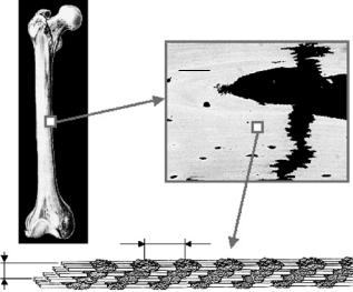
tissue. Such texture investigations have been carried out by X-ray di raction [50–52], and also by neutron scattering [53–56]. In the case of long bones, it was generally observed that the crystals are oriented with their longest dimension parallel to the long axis of the bone (which corresponds to the crystallographic c-axis of the hydroxyapatite). Moreover, this orientation gets more pronounced with age, which points to a continuous optimization of the bone’s nanostructure to withstand bending loads. Neutrons were useful in particular for anatomical studies with the aim to correlate the local mineral orientation to the stress patterns produced by specific loading situations in di erent types of bones [56]. In contrast to di raction using neutrons or X-rays – including also small-angle di raction to study for instance the axial periodicity of collagen – small-angle scattering (SAS) is usually understood as di use scattering, being sensitive to weakly ordered structures in the range from about 1 nm to about 100 nm [57–59]. Hence, structural parameters from the mineral particles in the collagen matrix of bone may be derived from SAS measurements. Small-angle X-ray scattering (SAXS) has been established and applied systematically in recent years to study size, shape, and orientation of mineral particles in bone [51, 59–66] and other mineralized tissue [29, 67–69],
214 P. Fratzl et al.
(a) |
(b) |
50 μm
~320 nm
(c)
~5 nm
Fig. 11.6. Hierarchical structure of compact bone in mammalian long bones. It consists typically of mineralized collagen fibrils (c, see also Fig. 11.2) which are assembled into a lamellar structure (b). The fibril orientation is typically rotating inside the lamellae in a plywood-like fashion [48, 49]. The typical size of mineral particles is a few nanometers, the diameter of fibrils a few hundred nanometers, the thickness of lamellae a few micrometers and the thickness of the cortical bone shell a few millimeters
and in the meantime it is a well-recognized analytical tool to study for instance medical questions related to bone diseases [70–77].
One of the consequences of the hierarchical architecture of bone (Figs. 11.6 and 11.7) is the fact that nanometer sized features such as the size and orientation of mineral particles may vary systematically throughout the tissue on a larger (typically micrometer-sized) scale. This introduces the technical di - culty that the nanometer-scale structures need, in principle, be characterized in a position-resolved way.
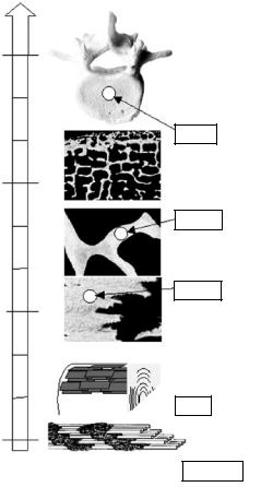
As an example, three distinct hierarchical levels are shown in Fig. 11.7 for human cancellous bone, i.e., the macroscopic anatomy of the vertebral body (mm), the size of single trabeculae ( 200 m) and the scale of single lamellae within the trabeculae ( 20 m). A very important impact of SAXS in recent years was indeed the possibility to use a beam size adapted to the hierarchy level of interest, allowing a position-resolved analysis by scanning of bone sections across the X-ray beam [59, 62, 64]. The principle of a scanning SAXS or scanning XRD experiments is very simple and is depicted schematically in Fig. 11.8. The specimen can be moved in two directions (x and y) perpendicular to the incoming X-ray beam. Scanning the sample through the beam while successively recording scattering patterns yields a two-dimensional image of
11 Complex Biological Structures |
215 |
m
2 mm
mm
200 μm
20 μm
μm
SAS
nm
Diffraction
Fig. 11.7. Hierarchical structure of mammalian cancellous bone. As compared to compact bone (Fig. 11.6), cancellous bone such as vertebra exhibits one more hierarchical level, namely a foam-like structure with struts of 100 – 300 m – the so called trabeculae – pointing preferentially into the direction of principal stresses. The structures at the nanometer scale can be investigated by small-angle scattering (SAS) and di raction techniques. Combination with scanning techniques using a beam adapted to the hierarchical level of interest (shown for three examples by the white circles) permits to image the nanostructure with a resolution corresponding to the beam size
these patterns. The lateral size of the beam – together with the specimen thickness, which should be adapted to the beam size – defines the spatial resolution of the scanning image. The scattering patterns are usually recorded in transmission geometry using a high resolution area detector as depicted in Fig. 11.8, allowing in some cases to record even both, the XRD and the SAXS signals simultaneously [78,79]. The evaluation of the scattering patterns
216 P. Fratzl et al.
Beam
Optical
Microscope
Beamstop
Sample
y
x
SAXS/XRD
Detector
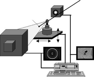
Fig. 11.8. Schematic picture of a scanning SAXS/XRD setup. An X-ray microbeam of lateral size D penetrates a sample with thickness D, defining an interaction volume of D3. The sample is scanned in two dimensions perpendicular to the primary beam with a step width of D, and successive SAXS and/or XRD patterns are collected for any scanning step using a high resolution area detector. To keep measurement time reasonable, scanning regions of interest at the sample can be selected with the help of an optical microscope. Data reduction to obtain one or several nanostructural parameters from every SAXS and/or XRD pattern, and matching of these parameters with real space images of the specimen (e.g., a light microscopy image) is presently done o ine after the experiment. In principle, fully automated data reduction, matching, and visualization may be possible online for certain application and will be a challenge for future developments
provides structural parameters from the nanometer level at every position of the scan. Such parameters may then be superimposed on a micrograph of the specimen, for instance on an X-ray scanning absorption image which has been taken prior to the scattering experiment [62,64,80]. Other options are to use an online, o -axis microscope such as in Fig. 11.8, or an o -line, on-axis microscope at a calibrated position with respect to the X-ray beam [79]. A scanning resolution in the order of about 200 m can be achieved using laboratory X-ray sources [62], but the most promising development is due to the high brilliance of third generation synchrotron radiation sources. X-ray microbeams of some micrometers diameter are nowadays available routinely at many dedicated microfocus beamlines (for instance at the beamline ID13 at the European Synchrotron Radiation Facility, ESRF, in Grenoble [79]), and current
11 Complex Biological Structures |
217 |
developments permit to reach the 100 nm regime in the near future. By building up scanning devices in combination with X-ray (or neutron) scattering it is thus possible, in principle, to cover the size-ranges from atomic dimensions to about 100 nm (by XRD and SAXS in reciprocal space) and above 100 nm (by moving the specimen stepwise across the beam in real space) in a single experiment. Moreover, the capability of imaging a specimen in the micrometer range opens the possibility of combining several experimental approaches. For instance, the combination of scanning SAXS with light microscopy and scanning electron microscopy (SEM) [63, 65], with FTIR-Microspectroscopy [81], and even with local imaging of mechanical properties using nano-indentation [67] has been demonstrated for the analysis of mineral particles in calcified tissue.
Scanning SAXS with 200 m Resolution:
Case Example of Cancellous bone
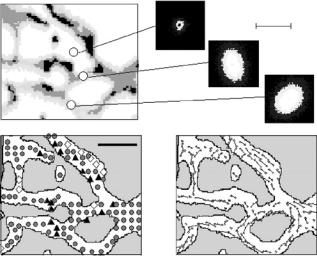
As shown in Fig. 11.7, the trabeculae in the spongiosa of human cancellous bone have a thickness of a few hundred micrometers. Thus, the mineral crystals in individual trabeculae can be investigated by scanning SAXS using a laboratory X-ray source with a beam diameter of about 200 m [62]. Figure 11.9 shows a typical result for a 200 m thick section of human vertebra embedded in polymethylmethacrylate. Figure 11.9a shows a scanning X-ray radiography taken by scanning the sample through the beam and measuring the transmitted intensity through the specimen at each position. The trabeculae appear as darker regions (higher absorption) in the radiography. Scattering patterns from selected areas on the sample are shown in Fig. 11.9b, where the scattered intensity is presented in a pseudo-gray scale, dark corresponding to low and bright to high intensity. Two of the scattering patterns taken at positions within the trabeculae have an elliptical shape, the third pattern (top left of Fig. 11.9b) was recorded in a region outside the trabeculae and shows isotropic background scattering from the resin.
An important nanostructural parameter derived from the SAXS patterns (Fig. 11.9b) is the ratio between the total volume and the total surface of mineral per unit volume of bone matrix, respectively [61]. It can easily be shown that for constant composition (around 50 vol% mineral content) this so called T -parameter is a measure for the smallest particle dimension, i.e., the thickness of the mineral platelets in bone. Figure 11.9c shows the values of the T -parameter obtained at various positions in the vertebra section. Smaller values of T at some outer trabecular regions can be attributed to younger bone formed by remodeling processes [63]. Two further parameters, which can directly be deduced from the orientation and the eccentricity of the elliptically shaped SAXS patterns, are the main orientation of the plate shaped mineral particles and their degree of alignment, respectively [61]. Particle orientation and degree of alignment are indicated by the direction and the length of the bars in Fig. 11.9d, respectively. It is seen that the long axis of the mineral
218 P. Fratzl et al.
(a) |
(b) |
4 nm−1 |
(c) |
(d) |
1 mm
Fig. 11.9. Example of scanning SAXS results from trabecular bone using an X- ray beam of 200 m size (from [62]). (a) shows scanning absorption image with the trabeculae in dark (high absorption) embedded in resin (bright = low absorption). SAXS patterns are shown in (b) for selected regions (indicated by circles) of the trabecular structure and in the resin. The length scale for the scattering vector q is also indicated and the scattered intensity is presented in a logarithmic pseudogray scale (dark = low intensity, bright = high intensity). (c) shows the contours of the trabeculae with the “average thickness” T of the plate-like mineral particles superimposed. T is calculated from the integrated intensity and the Porod constant
˜ −
P of the azimuthally averaged SAXS patterns, T = 4I/πP = 4Φ(1 Φ)/σ, where Φ and σ are the total volume and surface of mineral per unit volume of bone matrix, respectively. Triangles: T > 3.5 nm, circles: 3.5 nm < T < 3.0 nm, diamonds: T < 3.0 nm. (d) shows the orientation (direction of the bars) and the degree of alignment ρ (length of the bars) of the mineral particles with respect to the trabecular structure. The degree of alignment is a parameter varying between 0 and 1, where 0 corresponds to random orientation and 1 to a perfectly parallel alignment of the mineral platelets. The longest bars in (d) correspond to ρ ≈ 0.5
particles points preferentially into the direction of the trabeculae and such a behavior is found typical for human cancellous bone [63, 65].
Knowing that the trabecular orientation corresponds also to the principal stress directions, the optimization of the material bone with regard to its mechanical function at all levels is impressively demonstrated by the results in Fig. 11.9. A number of fundamental [63, 65, 66, 81], and medical questions [74, 75, 77] have in turn been studied on calcified tissue with the laboratory equipment providing 200 m scanning resolution. Very recently, the experiments on human cancellous bone have been extended to local 3D SAXS measurements within single trabeculae by applying an additional sample rotation [51]. This allows one to construct so called SAXS pole-figures,
11 Complex Biological Structures |
219 |
which quantify the 3D distribution of the local average habit plane of mineral platelets with respect to an external coordinate system (e.g., the trabeculae direction). By combining this SAXS pole-figure analysis with classical polefigure analysis using wide angle X-ray di raction from the bone mineral on exactly the same specimen positions, complementary information about the crystallographic texture (XRD) and the morphological texture (SAXS) could be gained [51].
Towards One Micrometer Position Resolution:
Lamellar Bone and Other Calcified Tissue
While for the investigation of the trabecular structure of bone a spatial resolution of about 200 m is su cient, many other structural features require a smaller beam size and consequently, synchrotron radiation comes into play. A first dedicated synchrotron setup for scanning SAXS of bone was designed to have a standard beam size of 20 m by using simple pinhole collimation [80]. Even though this was a rather ine cient way to create a microbeam, a flux of about 108 photons per second could be reached at the synchrotron radiation source ELETTRA, permitting SAXS scans on bone and other calcified tissues within some hours by carefully selecting small regions of interest [80]. An example for scanning SAXS with 20 m resolution is depicted in Fig. 11.10, showing an overlay of two scanning images from human cortical bone: in the background a backscattered electron image, and in the foreground an image of SAXS patterns from the same specimen positions exactly matched to the BE image [69, 80]. The di erent gray levels in the BE image correspond to di erent local mineral density (brighter gray level means higher mineral density) [82]. It is obvious that the mineral density is clearly lower in the osteons, which are the regions surrounding the elliptical holes [83]). The 2D image of SAXS patterns is overlaid to part the backscattered electron image, with the contours of the osteons indicated for better visualization. The SAXS intensity is clearly lower in the regions of the osteons, in qualitative agreement with the BEI images. The elliptical shape of the iso-intensity gray levels in the SAXS patterns indicates a preferred orientation of the mineral particles also in cortical bone, and their changing orientation suggests local changes of the morphological texture. It could indeed be shown that the particles are aligned in a cylindrical manner around the osteons [64]. Other examples where a position resolution of 20 m was used to study mineralized tissue concern the investigation of the interface region between bone and di erent types of mineralized cartilage [69] or the region near the edge of the mineralization front in mineralized turkey leg tendon [68]. Beside scanning SAXS, some first position resolved X-ray di raction experiments on calcified tissue with highest position resolution around – or even below – 1 m have recently been reported from the European Synchrotron Radiation Facility (ESRF) in Grenoble, such as for instance local investigations of archeological bone samples [84] or studies of reconstructed bone near prosthetic surfaces [85]. It has also been

220 P. Fratzl et al.
(a) |
100 |
μm |
|
(b)
Fig. 11.10. Scanning SAXS imaging of cortical bone. The background image (a) shows a backscattered electron image (BEI) from a 20 m thick section of cortical human bone (cross-section from a long bone such as in Fig. 11.6). The gray-levels in the BE image can be used to quantify the mineral density locally (qBEI) [82]. The overlaid image (b) consists of 2D SAXS patterns measured at exactly the corresponding specimen positions with 20 m beam size, and matched to the BE image. For clarity, the hollow channels and the borders of the osteons are indicated by black and gray colors in the image (b), respectively
demonstrated that local texture analysis in bone tissue is possible down to a few micrometers spatial resolution [86, 87]. In combination with scanning SAXS/XRD, this will open fascinating new possibilities to investigate the complex 3D-structure of lamellar bone at the level of single lamellae.
Scope for Position Resolved Neutron Scattering
The success and the rapid development of X-ray microbeams is a direct consequence of the extremely high brilliance of wiggler and undulator sources on the one hand, and the rapid development of X-ray optics on the other hand (see e.g., [79]). While the brilliance of neutron sources is generally low and will not increase considerably in the near future, all the focusing principles used for X-rays may in principle be applied with neutrons as well. When comparing di erent focusing devices, a quantitative description of the e ciency of a
11 Complex Biological Structures |
221 |
certain optical system to produce a small beam is given by the so called gain factor. This value describes essentially the ratio between the integrated flux in the focus of the optical system and the flux one would obtain by preparing a beam with the same size and divergence properties using conventional slit collimation. Several neutron optical devices were tested in recent years with similar gains as compared to X-ray optics, allowing thus to prepare su ciently intense neutron beams with a diameter below 100 m. For instance, a neutron beam of about 80 m diameter with a gain of 25 was reported using tapered capillaries [88] and similar gains were obtained by using compound refractive lenses [89]. Moreover, neutrons can be deflected in magnetic fields due to their magnetic moment. This has led to the construction of magnetic neutron lenses and focusing of a neutron beam with a gain of 35 using a permanent sextupol magnet has been reported [90]. Finally, even the feasibility of a sub-micron sized neutron (line) focus has been demonstrated recently by using a thin film wave-guide [91]. All these developments suggest that neutron beams with diameter in the order of 50–100 m may well be feasible in the future with su ciently high flux and low divergence for neutron di raction and for SANS experiments. We propose that such neutron “microbeams” could be used to establish scanning SANS as a complementary tool to scanning SAXS on a length scale of about 50–100 m. In particular the sensitivity of neutrons to the organic part of mineralized tissue would make position resolved neutron scattering on bone an attractive technique. In cancellous bone for instance, the detailed structure and arrangement of the collagen fibrils at the level of single trabeculae could be studied by this means with neutrons and complemented with the detailed structure of the mineral as obtained from X-rays.
References
1.J.L. Irigaray, H. Oudadesse, V. Brun, Biomaterials 22, 629–640 (2001)
2.D.J S. Hulmes, J. Struct. Biol. 137, 2–10 (2002)
3.P. Fratzl, Curr. Opin. Coll. Interf. Sci. 8, 32–39 (2003)
4.L. Knott, A.J. Bailey, Bone 22, 181–187 (1998)
5.T.J. Wess, A. Miller, J.P. Bradshaw, J. Mol. Biol. 213, 1–5 (1990)
6.T.J. Wess, L. Wess, A. Miller, Alcohol Alcohol 29, 403–409 (1994)
7.J.C. Hadley, K.M. Meek, N.S. Malik, Glycoconjugate J. 15, 835–840 (1998)
8.T.J. Wess, L. Wess, A. Miller et al, J. Mol. Biol. 230, 1297–1303 (1993)
9.P. Fratzl, A. Daxer, Biophys. J. 64, 1210–1214 (1993)
10.D.M. Maurice, J. Physiology-London 136, 263 (1957)
11.K.M. Meek, D.W. Leonard, Biophys. J. 64, 273–280 (1993)
12.G.F. Elliott, J.M. Goodfellow, A.E. Woolgar et al, J. Appl. Cryst. 11, 496–496 (1978)
13.G.F. Elliott, Z. Sayers, P.A. Timmins, J. Mol. Biol. 155, 389–393 (1982)
14.J.W. Regini, P.A. Timmins, G.F. Elliott et al, Biochim. Biophys. Acta 1620, 54–58 (2003)
15.H.D. Middendorf, R.L. Hayward, S.F. Parker et al, Biophys. J. 69, 660–673 (1995)
222 P. Fratzl et al.
16.H.D. Middendorf, A. Traore, L. Foucat et al, Physica B 276, 518–519 (2000)
17.H.D. Middendorf, U.N. Wanderlingh, R.L. Hayward et al, Physica A 304, 266– 270 (2002)
18.J.F.V. Vincent, in: Structural Biomaterials (Princeton University Press, Princeton, 1990)
19.N. Sasaki, S. Odajima, J. Biomech. 29, 1131–1136 (1996)
20.K. Misof, G. Rapp, P. Fratzl, Biophys. J. 72, 1376–1381 (1997)
21.P. Fratzl, K. Misof, I. Zizak et al, J. Struct. Biol. 122, 119–122 (1998)
22.N. Sasaki, N. Shukunami, N. Matsushima et al, J. Biomech. 32, 285–292 (1999)
23.V. Ottani, M. Raspanti, A. Ruggeri, Micron 32, 251–260 (2001)
24.R. Puxkandl, I. Zizak, O. Paris et al, Phil. Trans. R. Soc. Lond. B 357, 191–197 (2002)
25.F.H. Silver, Y.P. Kato, M. Ohno et al, J. Long-Term E ects Med. Implants 2, 165–195 (1992)
26.W. Folkhard, E. Mosler, W. Geercken et al, Int. J. Biol. Macromol. 9, 169–175 (1987)
27.E. Mosler, W. Folkhard, E. Knorzer et al, J. Mol. Biol. 182, 589–596 (1985)
28.W.J. Landis, K.J. Hodgens, J. Arena et al, Microscopy Res. Tech. 33, 192–202 (1996)
29.P. Fratzl, M. Groschner, G. Vogl et al, J. Bone Miner. Res. 7, 329–334 (1992)
30.W.J. Landis, J.J. Librizzi, M.G. Dunn et al, J. Bone. Miner. Res. 10, 859–867 (1995)
31.D.J.S. Hulmes, A. Miller, S.W. White et al, Int. J. Biol. Macromol. 2, 338–346 (1980)
32.J.W. White, A. Miller, K. Ibel, J. Chem. Soc. Faraday Trans. II 72, 435 (1976)
33.S.W. White, D.J.S. Hulmes, A. Miller et al, Nature 266, 421–425 (1977)
34.P. Fratzl, N. Fratzl-Zelman, K. Klaushofer, Biophys. J. 64, 260–266 (1993)
35.L.C. Bonar, S. Lees, H.A. Mook, J. Mol. Biol. 181, 265–270 (1985)
36.D.D. Lee, M.J. Glimcher, J. Mol. Biol. 217, 487–501 (1991)
37.S. Lees, L.C. Bonar, H.A. Mook, Int. J. Biol. Macromol. 6, 321–326 (1984)
38.S. Lees, D. Hanson, E. Page et al, J. Bone Miner. Res. 9, 1377–1389 (1994)
39.S. Lees, D.W.L. Hukins, Bone Mineral 17, 59–63 (1992)
40.S. Lees, H.A. Mook, Calcif. Tissue Int. 39, 291–292 (1986)
41.J.M.S. Skakle, R.M. Aspden, J. Appl. Cryst. 35, 506–508 (2002)
42.J. Orgel, A. Miller, T.C. Irving et al, Structure 9, 1061–1069 (2001)
43.D.J.S. Hulmes, T.J. Wess, D.J. Prockop et al, Biophys. J. 68, 1661–1670 (1995)
44.C.K. Loong, C. Rey, L.T. Kuhn et al, Bone 26, 599–602 (2000)
45.M.G. Taylor, S.F. Parker, P.C.H. Mitchell, J. Mol. Struct. 651, 123–126 (2003)
46.M.G. Taylor, S.F. Parker, K. Simkiss et al, Phys. Chem. Chem. Phys. 3, 1514– 1517 (2001)
47.S. Weiner, H.D. Wagner, Ann. Rev. Mater. Sci. 28, 271–298 (1998)
48.S. Weiner, T. Arad, I. Sabanay et al, Bone 20, 509–514 (1997)
49.A. Bigi, M. Burghammer, R. Falconi et al, J. Struct. Biol. 136, 137–143 (2001)
50.A. Ascenzi, E. Bonucci, P. Generali et al, Calcif. Tissue Int. 29, 101–105 (1979)
51.D. Jaschouz, O. Paris, P. Roschger et al, J. Appl. Cryst. 36, 494–498 (2003)
52.N. Sasaki, Y. Sudoh, Calcif. Tissue Int. 60, 361–367 (1997)
53.G.E. Bacon, P.J. Bacon, R.K. Gri ths, J. Appl. Cryst. 10, 124–126 (1997)
54.G.E. Bacon, P.J. Bacon, R.K. Gri ths, J. Anatomy 139, 265–273 (1984)
55.R.K. Gri ths, G.E. Bacon, P.J. Bacon, J. Anatomy 124, 253–253 (1977)