Neutron Scattering in Biology - Fitter Gutberlet and Katsaras

468 W. Doster

underlying the normal mode analysis of proteins [13, 14]. M¨ossbauer resonance spectra recording the motion of the heme group were analyzed using a “rugged” Brownian oscillator (BO) model [19]. Surprisingly the BO is not very popular among neutron experimentalists. Instead it is often assumed that protein residues perform free di usion inside a rigid sphere [20]. The oscillator model does not involve specific assumptions (which are hard to test) and provides a more general perspective. It allows us to pick up the discussion on time and length scales of chap. 19. An example of a Brownian mode analysis was discussed for phycocyanin by Hinsen et al. [21]. Neutron scattering probes the hydrogen atoms attached to the side chains and the main chain. We assume that the amino acid positional fluctuations follow approximately Eq. 20.1 and start with a one-dimensional model: V (x) = Kx2. The harmonic potential implies for the deviations a Gaussian probability distribution. The mean square displacements evolve at high damping monotonically toward an equilibrium value, the average thermal amplitude δ2 [21, 22]

The thermal amplitude amounts to δ2 = kBT /K. The relaxation rate is given by Γ0 = K/f and D = kBT /f may be interpreted as a di usion coe cient. Inserting Eq. 20.20 into Eq. 20.10, yields the following intermediate scattering function of the overdamped BO

The correlation function, IB(Q, t), exhibits several interesting features shown in Fig. 20.3. It is nonexponential in time, its e ective relaxation time depends on Q and it decays toward a finite plateau at long times the so-called elastic incoherent structure factor, EISF(Q).

Figure 20.3 shows an experimental intermediate scattering function derived from D2O-hydrated myoglobin [7, 8, 23] covering a wide Q-range. This experiment thus reflects essentially protein structural fluctuations. The harmonic oscillator model fits the data below Q = 2 ˚A−1. But the observed long-time plateau is much higher than predicted by the model at large Q. The spatial constraints of the protein-displacements are thus more severe than those of an isotropic harmonic potential.

The dashed line in Fig. 20.3 was obtained by assuming a two-dimensional harmonic oscillator (see below). The EISF(Q) decreases with increasing spatial resolution (Q) at fixed relaxation rate Γ0. Since IB(Q, t) is not a single exponential one obtains a Q-dependent average relaxation rate according to

470 W. Doster

with M¨ossbauer spectroscopy at Q = 7 ˚A−1 one should observe a much larger rate than for the same oscillator motion at Q = 2 ˚A−1 with neutron scattering.

20.6 The Visco-Elastic Brownian Oscillator

In our simple model we consider conformational fluctuations coupled to fast motions of the solvent, which acts as a heat bath. The BO model of Eq. 20.1 assumes a clear cut separation of time scales between heat bath coordinates and Brownian motion. This allows treating the random force as a δ-correlated Gaussian process (white noise) and the friction coe cient to be time independent. Protein structural fluctuations observed with neutron scattering occur, however, on time scales comparable to solvent dynamics. Thus one has to take into account explicitly the spectrum of random forces, which leads to a time-dependent friction according to the fluctuation-dissipation theorem. The Mori–Zwanzig theory provides an algorithm for the equation of motion, which yields for the density correlator ΦQ(t) a generalized oscillator equation containing a time dependent friction kernel m(t), reflecting the slow force correlations [3, 24, 25]. Ω and γ0 denote a generalized frequency and a regular

damping coe cient:

t

¨ 2 ˙ 2 − ˙

ΦQ(t) + Ω ΦQ(t) + γ0ΦQ(t) + Ω dt m(t t )ΦQ(t ) = 0 . (20.24)

0

A general solution to Eq. 20.24 can be given in the frequency domain for the spectrum S(Q, ω) [3, 18]

√

“Im” denotes “imaginary part of” and i = −1. M (Q, ω) represents a generalized friction kernel, which can be decomposed into a Newtonian friction γ0 (collisions) and a slow relaxing part mps(Q, ω) due to protein solvent coupling [25]

To illustrate the basic features of visco-elasticity, we introduce Maxwell’s relaxation model. The spectrum of force correlations is Lorentzian in shape, corresponding to an exponential decay of the force correlations [25, 26]

F is the amplitude and τ denotes the characteristic time of the relaxing friction, which is proportional to the viscosity η = G∞ · τ . G∞ is the high frequency shear modulus of the liquid. The real part of mps(ωτ ) contributes to the elastic modulus, while the imaginary part yields a frequency-dependent friction coe cient, f (τ, ω) mps(τ, ω):

Fig. 20.5. Real (dashed ) and imaginary part of ωmps(ω) according to Eq. 20.28

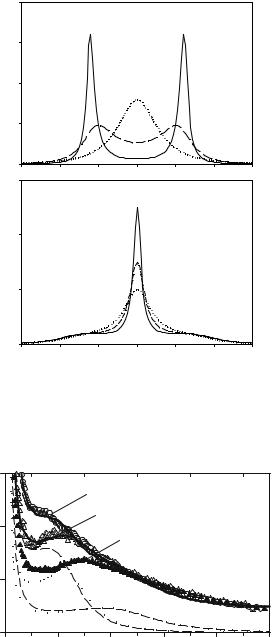
The dissipation rate thus assumes a maximum at ωτ = 1. The friction coe cient vanishes in both limits, f (τ → ∞) τ −1 and f (τ → 0) τ at fixed ω as shown in Fig. 20.5. The visco-elastic system thus turns into an elastic solid if the correlation time and thus the viscosity of the heat bath diverges. The same arguments apply to a variation of the frequency at fixed τ . For the simple BO increasing friction will always enhance the viscous properties. As shown in Fig. 20.6a, increasing the damping constant γ leads to a downshift and broadening of the resonance maxima. In the overdamped regime only a narrow central line will remain. In the visco-elastic case, the friction coe cient declines with increasing frequency. Thus even at high viscosity or large τ , an oscillation will persist since τ ω0−1.

Experimental neutron scattering spectra behave very much like those in Fig. 20.6b. The vibrational feature near 3 meV has been termed the “boson peak,” and involves low frequency oscillations of the protein structure. It is most prominent for large τ (low temperature and high viscosity) and becomes “overdamped” at high temperatures, when the viscoelastic relaxation times are comparable to ω0−1. A visco-elastic analysis was performed with neutron scattering data of myoglobin [8, 26]. The low-temperature spectrum (150 K) was adjusted to Eq. 20.25, assuming two oscillators as shown in Fig. 20.7. Then by decreasing only the visco-elastic relaxation time τ , the spectrum at 300 K could be simulated. Note that the maximum of Ω2 is nearly independent of τ in contrast to Ω1. Note also the di erence in position of the boson peak at low temperature between dry and hydrated myoglobin [27].

In this particular experiment we were interested whether the energy of photons absorbed by the heme group of myoglobin was channeled into low frequency vibrations near 30 cm−1. Following a laser pulse at 532 nm, we found a simultaneous emission in the far infrared below 50 cm−1, suggesting exactly this [26]. The self-friction kernel mss(Q, ω) of simple liquids has been calculated on a molecular basis by mode-coupling theory (MCT) [3]. MCT predicts a self-induced structural arrest of the liquid, when the density, depending on

472 W. Doster

Visco-elastic oscillator

2

S(w)

hw (meV)

Fig. 20.6. (a) Spectrum of a BO: underdamped regime (full line), intermediate (dashed ) and the overdamped case (dotted ), parameters in meV: ω0 = 2.4, γ = 0.5, 3.0, 6.0. (b) spectrum of visco-elastic oscillator (Eq. 20.24), the relaxation time τ increases from dotted, dashed to full line, F = 1.7, γ = 0.5, 1/τ = 0.5, 1.0, 2.0 meV. The broadening at ω = 0 is sometimes called the Mountain line

Fig. 20.7. Spectrum of dry and hydrated myoglobin and visco-elastic analysis assuming two oscillators, ω0 = Ω1, Ω2 [26]

.

Time (ps)

Fig. 20.8. Schematic intermediate scattering function of the generalized MCToscillator showing a two-step decay due to fast local (β-process) and slow collective motions (α-process). The oscillatory feature at short times generates the boson-peak in the frequency domain

temperature, pressure, and number concentration, exceeds a critical value. The signature of the glass-transition are nonvanishing density correlations and thus a finite value of the long time intermediate scattering function as shown in Fig. 20.8. MCT approximates the so-called cage e ect, each particle is surrounded by a cage of nearest neighbors. Escape out of the cage (the α-process) constitutes the first step leading to long-range di usion, which is the essence of the liquid state.

Fast local motions (β-processes) can also occur in the glass, but their amplitude (not their rate!) decreases when the density increases. In water, β-processes include hydrogen bond fluctuations and reorientational motions while the α-process involves translation. The glass transition is accompanied by a diverging α-relaxation time, the cage becomes a trap. This reasoning also applies to protein hydration water, which forms a glass at low temperatures [28]. As mentioned in Sect. 20.1, protein residues in a native structure are highly constrained and cannot perform long-range translational displacements. A native protein is not in a liquid state and thus cannot exhibit a liquid to glass transition. However, the protein residues are frictionally coupled to hydration water, which performs a self-induced glass transition at low temperatures [28]. Consequently, water-coupled protein motions will also be arrested because the plasticizer is arrested. Vitrification can also be achieved by cosolvents which seems to be equivalent to dehydration, as Fig. 20.1 shows. Sticking to the generalized oscillator concept, one may introduce the dynamic protein–solvent interactions at the level of the friction kernels

474 W. Doster

The internal friction due to water-decoupled structural motions is represented by mp. With this kernel, water-coupled structural fluctuations will freeze in parallel with the hydration water and behave liquid-like at high temperature. Proceeding in this direction, we have to study the properties of hydration water, which is a true liquid.

20.7 Moment Analysis of Hydration Water

Displacements

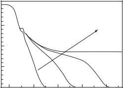
In the following we analyze experiments performed with H2O-dehydrated myoglobin in the range of 0.35 g g−1 degree of hydration. At this level, most of the water is in close contact with the protein surface. The hydration water does not freeze forming ice at low temperatures, instead it vitrifies forming an amorphous structure [28]. Figure 20.9 shows the intermediate scattering function I(Q, t) of water in the hydration shell of H2O-hydrated myoglobin at various Q-values. It is obtained by Fourier-transforming the spectral function, S(Q, ω). The amplitude of the fast component at 0.3 ps increases with Q indicating that this component is highly localized. It reflects damped translational oscillations of water molecules. The rate constant of the second process increases with Q (spatial resolution) [29].

This is a characteristic feature of translational di usion. One expects an exponential correlation function with a characteristic rate 1/τ = Q2 · D with di usion constant D. Instead we observe a stretched-exponential decay where

Fig. 20.9. Intermediate scattering function of myoglobin hydration water at 0.35 g H2O per g protein and fits to a stretched exponential function (IN6, ILL) [29]

the di usion coe cient is Q-dependent [29]

The stretched behavior, (β < 1) results from partially localized water molecules at the protein surface. The second equality in Eq. 20.30 refers to a more general property of I(Q, t), which may be expanded in terms of the second and higher moments of the displacement distribution function according to Eq. 20.6

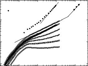
Adjusting the data to a fourth-order polynom yields the second and the fourth moment of the displacement distribution function G(r, t). In practice one has to account for multiple scattering corrections A0(t) [29,30]. Figure 20.10 shows the mean square displacements of protein interfacial water in comparison with bulk water [29]. The data on bulk water by Brockhouse and collaborators provided the first information on fast motions in a liquid using neutron spectroscopy [31]. After the initial rise due to vibrational dephasing, the dis-

sion coe cient of water, D = 2.45 · 10−5 cm2 s−1.

Note the sublinear regime near 1 ps, which reflects the motion of water molecules inside the cage formed by its nearest neighbors. For interfacial water the sublinear range is drastically extended, it takes about 100 ps to reach the

t (ps)

Fig. 20.10. Time-resolved displacements of bulk water and myoglobin interfacial water at 0.4 g D2O per g protein versus temperature (IN6, ILL; full circles: IN15, ILL)

476 W. Doster

1.0

Hydration water

T (K) =

270

0.8 300

320

)(t 2

(tC )/B

0.6

Gauß

0.4

t (ps)

Fig. 20.11. Gauss deviation (fourth moment) of the hydration water displacement distribution versus time of myoglobin (0.35 g g−1)

regime of regular di usion. The protein thus enhances the cage e ect leading to partially localized water states. With decrease in temperature the cage becomes a trap. The extended plateau at 180 K is the signature of a solid state. Structural arrest is achieved continuously as the temperature decreases, which excludes discontinuous transitions such as ice formation.

Figure 20.11 shows the time-dependent fourth moment of the water displacement distribution which is larger than the Gaussian value of 0.5. This indicates that water displacements near the protein surface occur preferentially along a preferred direction. However, at times above 100 ps, the Gaussian value is reestablished, consistent with the observed linear time dependence of the second moment, Fig. 20.10.

20.8 Analysis of Protein Displacements

We now turn to protein motions. As mentioned earlier the relevant spatial information is contained in the Q-dependence of the intermediate scattering function I(Q, t). Figure 20.12 shows this function at fixed tres = 50 ps versus temperature for myoglobin in three environments of Fig. 20.1.

A linear (Gaussian) behavior of ln[I(Q)] versus Q2, is observed at low temperatures reflecting vibrational displacements. But above 200 K nonGaussian deviations, first described in [7] become significant. Nearly identical scattering functions are found for the dry and vitrified sample, pointing to similar intramolecular motions. The addition of water has a significant e ect on the

Fig. 20.12. Long time value of I(Q, t ≈ 50 ps) versus Q and temperature for dry myoglobin. Selected data of vitrified and hydrated myoglobin are also shown, line: fit to Eq. 20.18, instrument: IN13, ILL

density correlations, indicating water-assisted protein displacements. The simplest model, which fits the data, is a displacement distribution composed of two Gaussians [32, 33]

" # " #

I(Q, T, tfix) = A1 · exp(−Q2 x21 /2) + A2 · exp(−Q2 x22 /2). (20.32)

Figure 20.13 shows the second moments of the two Gaussian components determined on absolute scale [7, 10].

The first component has a plateau at low temperatures given by the protein zero point vibrations (0.014(±0.002) ˚A2. This component shows harmonic behavior across the whole temperature range in the case of the dehydrated and the vitrified system. However, in the hydrated system an additional increase occurs above 240 K due to water-assisted motions. In contrast the second component emerges above 150 K and leads to a nonlinear enhancement in the total displacements independent of the protein environment. Figure 20.14 shows that the corresponding displacement distribution of hydrated myoglobin at fixed time versus temperature, 4π r2G(r, T, t = 50 ps). Component 1 broadens with increasing temperature due to vibrational motions. But above 240 K the maximum is shifting and the width increases. This e ect points to small scale continuous motions. It is seen only with hydrated samples. In contrast, component 2 is observed in all samples independent of the protein environment. It has its maximum near 1.5 ˚A, indicating large scale excursions.

What is the molecular nature of the two types of motions? Several authors have emphasized the relevance of dynamical heterogeneity in the context of neutron scattering experiments [33, 34]. With neutron scattering we probe, because of their large cross-section, the trajectories of nonexchangeable