Neutron Scattering in Biology - Fitter Gutberlet and Katsaras
.pdf22 Structure and Dynamics of Model Membrane Systems |
529 |
29.T.L. Kuhl, J. Majewski, J.Y. Wong, S. Steinberg, D.E. Leckband, J.N. Israelachvili, G.S. Smith, Biophys. J. 75 (1998), 2352
30.G.P. Felcher, R.J. Goyette, S. Anastasiadis, T.P. Russell, M. Foster, F. Bates, Phys. Rev. B 50 (1994), 9565
31.S. Langridge, J. Schmalian, C.H. Marrows, D.T. Dekadjevi, B.J. Hickey, Phys. Rev. Lett. 85 (2000), 4964
32.Z.X. Li, J.R. Lu, R.K. Thomas, A. Weller, J. Penfold, J.R.P. Webster, D.S. Sivia, A.R. Rennie, Langmuir 17 (2001), 5858
33.W. Helfrich, Z. Naturforsch. 28c (1973), 693
34.L. Ning, C.R. Safinya, R. Bruinsma, J. Phys. II France 5 (1995), 1155
35.N. Lei, PhD thesis, Rutgers, 1993
36.A. Caill´e, C. R. Acad. Sci. 274 (1971), 891
37.R. Holyst, D.J. Tweet, L.B. Sorensen, Phys. Rev. Lett. 65 (1990), 2153
38.J. Als-Nielsen, J.D. Litster, R.J. Birgenau, M. Kaplan, C.R. Safinya, Phys. Rev. B 22 (1980), 312
39.S.K. Sinha, J. Phys. III (France) 4 (1994), 1543
40.A. Schreyer, R. Siebrecht, U. Englisch, U. Pietsch, H. Zabel, Physica B 248 (1998), 349
41.T. Salditt, T.H. Metzger, J. Peisl, Phys. Rev. Lett. 73 (1994), 2228
42.T. Salditt, D. Lott, T.H. Metzger, J. Peisl, G. Vignaud, P. Høghøj, O. Sch¨arpf,
P.Hinze, R. Lauer, Phys. Rev. B 54 (1996), 5860
43.R. Cubitt, G. Fragneto, Appl. Phys. A 74 (2003), 329
44.M. Vogel, PhD thesis, Universit¨at Potsdam, 2000
45.T. Salditt, M. Vogel, W. Fenzl, Phys. Rev. Lett. 90 (2003), 178101
46.C. Ollinger, D. Constantin, J. Seeger, T. Salditt, Europhys Lett. 71 (2005), 311
47.S. Ludtke, K. He, H. Huang, Biochemistry, 34 (1995), 16764
48.S.J. Ludtke, K. He, W.T. Heller, T.A. Harroun, L. Yang, H.W. Huang, Biochemistry 35 (1996), 13723
49.L. Yang, T.M. Weiss, R.I. Lehrer, H.W. Huang, Biophys. J. 79 (2000), 2002
50.T. Bayerl, Curr. Opin. Coll. Interface Sci. 5 (2000), 232
51.S. Paula, A.G. Volkov, A.N. Van Hoek, T.H. Haines, D.W. Deamer, Biophys.
J.70 (1996), 339
52.W. Pfei er, Th. Henkel, E. Sackmann, W. Knorr, Europhys. Lett. 8 (1989), 201
53.S. K¨onig, T.M. Bayerl, G. Coddens, D. Richter, E. Sackmann, Biophys. J. 68 (1995), 1871
54.E. Endress, H. Heller, H. Casalta, M.F. Brown, T.M. Bayerl, Biochemistry 41 (2002), 13078
55.A.A. Nevzorov, M.F. Brown, J. Chem. Phys. 107 (1997), 10288
56.S.H. Chen, C.Y. Liao, H.W. Huang, T.M. Weiss, M.C. Bellisent-Funel, F. Sette, Phys. Rev. Lett. 86 (2001), 740
57.M.C. Rheinst¨adter, C. Ollinger, G. Fragneto, F. Demmel, T. Salditt, Phys. Rev. Lett. 93 (2004), 108107
58.M.C. Rheinst¨adter, C. Ollinger, G. Fragneto, T. Salditt, Physica B 350 (2004), 136
59.F. Demmel, A. Fleischmann, W. Gl¨aser, Nucl. Instrum. Methods Phys. Res., Sect. A 416 (1998), 115
60.A. Spaar, T. Salditt, Biophys. J. 85 (2003), 1576
61.F.Y. Chen, W.C. Hung, H.W. Huang, Phys. Rev. Lett. 79 (1997), 4026
62.C.Y. Liao, S.H. Chen, F. Sette, Phys. Rev. Lett. 86 (2001), 740
63.T.M. Weiss, P.-J. Chen, H. Sinn, E.E. Alp, S.H. Chen, H.W. Huang, Biophys.
J.84 (2003), 3767
530 T. Salditt, M.C. Rheinst¨adter
64.M. Tarek, D.J. Tobias, S.-H. Chen, M.L Klein, Phys. Rev. Lett. 87 (2001), 238101
65.P.C. Mason, J.F. Nagle, R.M. Epand, J. Katsaras, Phys. Rev. E 63 (2001), 030902(R)
66.A.F. Xie, R. Yamada, A.A. Gewirth, S. Granick, Phys. Rev. Lett. 89 (2002), 246103
67.P. Sens, M.S. Turner, J. Phys II. France 7 (1997), 1855
68.P. Sens, M.S. Turner, Phys. Rev. E 55 (1997), R1275

23
Subnanosecond Dynamics of Proteins
in Solution:
MD Simulations and Inelastic Neutron
Scattering
M. Tarek, D.J. Tobias
23.1 Introduction
Complete understanding of protein function requires knowledge of their structure, energetics, and dynamics at the atomic level. To probe dynamics, inelastic neutron scattering (INS) has emerged as a powerful tool allowing the space and time-resolved study of a wide spectrum of motions in biomolecules taking place in the subpicosecond to multinanosecond timescales [1–8]. The ranges of energy and momentum transfers accessible on presently available neutron spectrometers correspond closely to the lengths and sizes of Molecular Dynamics (MD) simulations that are feasible nowadays for biological molecules (cf. Fig. 23.1). Therefore, simulations are a potentially valuable tool for interpreting neutron data on biomacromolecules, and similarly neutron scattering experiments can be used to verify results from MD calculations in a previously inaccessible time regime, and this has a direct impact on the rapidly growing area of computational biology.
Due to experimental limitations, neutron scattering was initially used primarily to study protein dynamics in powder environments in order to balance the trade-o between maximal scattered neutron flux and minimal data collection time. Despite their widespread usage in the food and pharmaceutical industries [9–11] or in research applications, very little is known about the organization and interactions of the protein molecules in these powders. Hydrated samples are usually prepared by adding a prescribed amount of water to a dry lyophilized powder. Lyophilization consists of freeze–drying an aqueous solution of the protein under vacuum. Although reversible by full hydration, lyophilization is known to induce changes in protein structure and make proteins more rigid [12]. Thus there is some concern that partially hydrated powder samples may contain a certain amount of nonnative structure and therefore, the scattering data taken on powders may not be truly representative of native functioning proteins.
 Larger distances
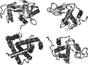
23 MD simulations and Inelastic Neutron Scattering |
533 |
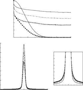
of the INS data has been considered in some studies [19], the validity of the assumptions made remains unclear. The contribution from the overall motion has simply been ignored in several other studies. This stems mainly from the fact that it is counterintuitive that the overall translational and rotational motion of globular proteins in solution, known from light scattering and NMR measurements to be appreciable only on the nanosecond timescale, have an e ect on motion probed with neutrons on the tens of picoseconds timescale.
Here we extend our MD simulation studies to investigate the dynamics of proteins in solutions, at low to moderate concentrations. We have two objectives. First, we use the simulation results to provide support to the assumptions made in experimental data reduction. Second, we use the atomistic modeling to characterize the changes in the internal dynamics of a protein upon going from low hydration to high hydration. To these ends we present results obtained from a series of simulations of four globular proteins in solution: Ribonuclease A (RNase A), myoglobin (Myo), lysozyme (Lys), α-lactalbumin (α-Lact) (Fig. 23.2). In the case of RNase A, we compare results from the solution simulation with previous simulations in powder environments both at very low and intermediate hydrations.
The purpose of this chapter is not to present a comprehensive review on probing dynamics of proteins with neutron scattering (up-to-date references are reported in several chapters of this book) and MD simulations. Rather, we focus on a few examples to demonstrate the utility of combining neutron scattering experiments and MD simulations in order to elucidate the dynamical
Ribonulease |
Lysozyme |
Myoglobin |
A-Lactalbumin |
Fig. 23.2. Ribbon representation of the four proteins studied (Protein Data Bank access codes in parentheses): Bovine pancreatic Ribonuclease (7RSA) [21], sperm whale Myoglobin (1MBC) [22], human α-Lactalbumin (1HML) [23], and hen egg white Lysozyme (194L) [24]
534 M. Tarek et al.
behavior of proteins in solution at the atomic level. The chapter is organized as follows. First, we describe the computational approaches used in the simulations, including the system setup, simulation protocols, and the methods used for analysis of the results. Next, we discuss the MD simulations results in comparison to neutron scattering measurements performed on proteins in powder and solution environments, and conclude with a detailed description of the internal dynamics of proteins in the di erent environments.
23.2 MD Simulations
Molecular dynamics refers to a family of computational methods aimed at simulating macroscopic behavior through the numerical integration of the classical equations of motion of a microscopic many-body system. Macroscopic properties are expressed as functions of particle coordinates and/or momenta, which are computed along a phase space trajectory generated by classical dynamics. The underlying assumption is that over long times the system will reach an equilibrium state, in which time averages can be equated to statistical ensemble averages. When performed under conditions corresponding to laboratory scenarios, molecular dynamics simulations can provide a detailed view of the structure and dynamics at the atomic and mesoscopic levels that is not presently accessible by experimental measurements. They can also be used to perform “computer experiments” that could not be carried out in the laboratory, either because they do not represent natural behavior, or because the necessary controls cannot be achieved. Lastly, MD simulations can be implemented as simple test systems for condensed matter theory. In order to realize this wide spectrum of applications, several issues concerning system modeling, dynamical generation of statistical ensembles, and e cient numerical integrators, must be considered.
MD simulations use information (positions, velocities or momenta, and forces) at a given instant in time, t, to predict the positions and momenta at a later time, t + ∆t, where ∆t is the time step, usually taken to be constant throughout the simulation. Numerical solutions to the equations ofmotion are thus obtained by iteration of this elementary step. The most popular algorithms for propagating the equation of motion, or “integrators,” are based on Taylor expansions of the positions (see [25] for a survey). A popular approach to increasing the time step in MD simulations of molecular systems is to use holonomic constraints to freeze the motion of the highest frequency bonds, or all of the bonds altogether. This is acceptable because the bond stretching motion is e ectively decoupled from the other degrees of freedom that are typically of greater interest. There are a variety of algorithms (e.g., shake, rattle) for solving the appropriate constraint equations and integrating the equations of motion (see [25]).
The utility of the constraint method rests on the fact that the fastest degrees of freedom place an upper bound on the time step, and the time step can therefore be increased if the fastest degrees of freedom are eliminated.
23 MD simulations and Inelastic Neutron Scattering |
535 |
A more general approach is based on the premise that the forces associated with di erent degrees of freedom evolve on di erent timescales, and the slower forces do not need to be computed as often as the faster forces. It turns out, for molecular systems, that the fastest forces, those associated with intramolecular interactions, require the least computational e ort to evaluate (O(N )), while the slowest forces, those associated with nonbonded interactions, require the most computational e ort (O(N 2)). Thus, in the interest of computational e ciency, it is clearly advantageous to calculate the rapidly evolving forces at each elementary time step, and calculate only the slowly evolving forces at a larger time interval that is several times the elementary time step. This is the essence of multiple time step MD, which is used in most MD simulations of biomolecules these days (see [26] for a review and technical details).
To date, most MD simulations have been driven by forces that were derived from assumed, empirical potentials (for a detailed overview of commonly used empirical potentials, see [27]). Although the number and nature of the potential energy terms varies from one application to the next, the potential for an arbitrarily complicated molecule such as a biopolymer is generally written as the sum of “bonded” and “nonbonded” terms. The bonded terms include energy penalties, usually represented by harmonic potentials, for deforming chemical bonds and the angles between bonds from their equilibrium values as well as periodic potentials to describe the energy change as a function of torsion (dihedral) angle about rotatable bonds. The bonded terms are usually taken to be diagonal, i.e., there are no terms describing coupling between deformations of bonds and angles, bonds, and torsions, etc. These o -diagonal terms are important for accurate reproduction of vibrational properties, as are anharmonic terms (e.g., cubic, quadratic). The nonbonded terms, as the name suggests, describe the interactions between atoms in di erent molecules, or interactions within a molecule that are not completely accounted for by the bonded terms, i.e., they are separated by more than two bonds. The nonbonded terms are typically assumed to be pairwise-additive functions of interatomic separation, r, and include van der Waals interactions and Coulomb interactions in polar or charged molecules in which the charge distribution is represented by partial charges (usually placed on the atoms). The van der Waals interactions, commonly modeled by the Lennard–Jones potential, include a term that is strongly repulsive (exponential or inverse 12th power of r), and a weakly attractive dispersion term (e.g., inverse sixth power of r, representing the induced dipole-induced dipole interaction).
An important aspect of performing simulation studies is to calculate experimentally measurable properties for comparison with measurements made at particular thermodynamic state points. Most experiments are carried out under the conditions of constant temperature and either constant pressure or volume, e.g., in the isobaric–isothermal or canonical statistical mechanical ensembles. However, integration of Newton’s equations of motion generates trajectories at constant volume and energy, i.e., in the microcanonical ensemble. Several techniques for generating trajectories in ensembles other than the

536 M. Tarek et al.
microcanonical ensemble have been developed (see [25] for an overview). The most powerful techniques are based on the concept of an “extended system” (ES), in which the atomic positions and momenta are supplemented by additional dynamical variables representing the coupling of the system to an external reservoir (see [26] for a review and technical details).
23.2.1 Systems Set-up and Simulations
The simulations were all initiated from crystal structures. For each system, the protein monomers were first solvated in a well-equilibrated water box. After energy minimization, a constant volume and temperature (300 K) equilibration run was followed by constant pressure (1 atm.) and constant temperature (300 K) runs. The powder simulations have been previously described in length [13–16]. We therefore only briefly outline here the set up procedure and run parameters. The powder representations of RNase A each contain eight protein molecules replicated by periodic boundary conditions (so that they are actually polycrystalline) constructed from four unit cells (a 2a × 2b × c lattice) of the monoclinic crystal with the water molecules removed. First, a constant volume MD run at 500 K was used to produce non-native, disordered configurations on the surfaces of the protein molecules. This was followed by a constant pressure run at 300 K during which the system contracted, enabling the protein molecules to interact with their neighbors and periodic images, followed this. The system was then hydrated up to hydration levels of h = 0.05 g and h = 0.42 g D2O per gram protein to correspond to lowand highhydration experiments by adding 280 and 2,188 water molecules, respectively.
A summary of the simulated protein in solution systems is given in Table 23.1. The CHARMM22 force field [28] was used. Three-dimensional periodic boundary conditions were applied and the Ewald sum was used to calculate the electrostatic energies, forces, and virial in all of the simulations. The Lennard–Jones interactions and the real-space part of the Ewald sum were smoothly truncated at 10 ˚A, and long-range corrections to account for the neglected interactions were included in the energies and pressures [25]. The reciprocal space part of the Ewald sum was calculated using the smooth particle mesh method [29]. The extended system Nos´e–Hoover chain method [30] was used to the control the temperature in all of the simulations, with separate thermostat chains for the water and protein molecules. The constant
Table 23.1. Characteristics of the simulated systems
|
|
no. of protein |
no. of α domains |
box/ |
no. of water |
protein |
PDB |
residues/atoms |
β strands |
˚3 |
) molecules |
dimensions (A |
|||||
Ribonuclease A |
7RSA |
124/1,144 |
3/9 |
57 × 52 × 40 |
3,453 |
Lysozyme |
194L |
129/1,141 |
4/3 |
56 × 48 × 78 |
6,461 |
Myoglobin |
1HBC |
153/1,404 |
9/0 |
57 × 52 × 40 |
3,290 |
α-Lactalbumin |
1HML |
142/1,102 |
4/3 |
58 × 50 × 80 |
4,655 |
23 MD simulations and Inelastic Neutron Scattering |
537 |
pressure simulations were carried out in a fully flexible simulation box by using the extended system algorithm of Martyna et al. [31]. A multiple time step algorithm [32] was used to integrate the equations of motion with a 4 fs time step. The lengths of bonds involving H/D atoms were held fixed by using the shake/rattle algorithm [33, 34].
23.2.2 Generating Neutron Spectra
MD simulations produce phase-space trajectories that consist of the positions and momenta of all the atoms in the system as a function of time. Here, we focus on quantities related to incoherent neutron scattering measurements that probe motions of hydrogen atoms on picosecond timescales. Neutron spectroscopy experiments essentially measure the total dynamic structure factor, Smeas(Q,ω), in which Q and ω are the momentum and energy transfers, respectively. Because the incoherent scattering length of hydrogen is an order of magnitude larger than the scattering lengths of all the other atoms in proteins and water (D2O) molecules, for the systems of interest here, the scattering is primarily incoherent, and hence Stotmeas(Q,ω) = Sincmeas(Q,ω). The incoherent dynamical structure factor may be written as the Fourier transform of a time correlation function, Iinc(Q,t) the intermediate scattering function
|
|
|
1 |
|
∞ |
|
Sinc(Q, ω) = |
|
−∞ Iinc(Q, t)e−iωt , |
(23.1) |
|||
2π |
||||||
Iinc(Q, t) = |
1 |
|
|
e−iQ·rj (0)eiQ·rj (t) . |
(23.2) |
|
|
|
|
||||
|
|
|
|
|||
N |
j |
|
||||
Here rj is the position operator of atom j, or, if the correlation function is calculated classically, as in an MD simulation, rj is a position vector, and the angular brackets denote an average over time origins and scatterers. Iinc(Q, ω) can be directly computed from an MD trajectory and Fourier transformed (FT) to a ord Sinc(Q, ω). Note that we have left out the prefactor corresponding to the square of the scattering length. This is convenient in the case of a single dominant scatterer because it gives I(Q, 0) = 1 and normalized to unity. The Iinc(Q, t) (and their corresponding spectra) reported in this paper are “powder averages” computed at eight randomly chosen scattering vectors with |Q| = Q.
Intermediate scattering functions in proteins do not decay completely on the timescale accessible to most experiments. A direct Fourier transform is therefore not appropriate. A window function is generally used in such cases, and the results may still be accurately compared to experiment if one considers the proper mathematical form for the window function. The best is that corresponding to the resolution function of the instrument.
In practice, the spread in energies of the neutrons incident on the sample results in a finite energy resolution, and the measured spectrum Sinc,meas(Q, ω)