Neutron Scattering in Biology - Fitter Gutberlet and Katsaras

resolution of 100 eV, the dynamical structure factor contains contributions from motions that are longer the σ. Thus, it is inappropriate to use σ as a fixed time interval for computing time averages if the objective is a quantitative comparison with neutron scattering data.

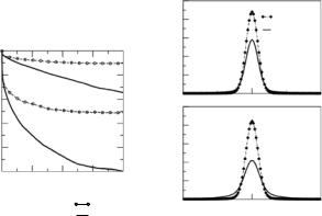
Interpretation of Sincmeas(Q, ω) in terms of atomic dynamics requires models for the di usive motions. QENS spectra for proteins and other disordered, condensed phase systems are often interpreted in terms of di usive motions that give rise to an elastic line with a Q-dependent amplitude, and a series of Lorentzian quasi-elastic lines with Q-dependent amplitudes and widths, i.e.,

where Li(Γi(Q), ω) is a Lorentzian centered at ω= 0 with half-width-at-half- maximum Γi(Q)

The amplitudes of the elastic scattering, A0(Q), the elastic incoherent structure factor (EISF), provides information on the geometry of the motion, while the line widths are related to the time scales (broader lines correspond to shorter times). The Q and ω dependence of these spectral parameters are commonly fitted to dynamical models for which analytical expressions for Sincdi (Q, ω) have been derived (e.g., jump di usion, di usion-in-a-sphere, etc.), a ording di usion constants, jump lengths, residence times, etc. characterizing the motion described by the models [35]. Such models can be scrutinized using the exquisite detail contained in MD simulation trajectories.

23.3 Overall Protein Structure and Motion in Solution

To assess the ability of the simulations to maintain the correct internal structure of the protein molecules, we have computed the root-mean squared deviations (r.m.s.ds) of the Cα positions in the simulations from the corresponding crystal structure. The Cα atoms define the backbone of the protein molecule. In each case the r.m.s.ds had converged (to values between 1.0 and 1.5 ˚A) before the averaging period, in the sense that they exhibited small fluctuations in time about their averages, which were not drifting. The results indicate that the overall protein structure is reasonably well maintained during the simulations. When making such comparisons it is important to keep in mind that some deviation from the crystal structure is expected because the intermolecular contacts present in the crystal are absent in solution. We have also computed the time evolution of the radius of gyration Rg of the molecules during the simulations, where Rg is computed using all the protein atoms ac-

cording to the standard formula: Rg = N mi(ri −rcom)2/ mi , rcom being

i

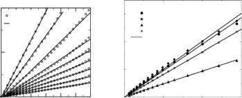
Fig. 23.5. Analysis of the overall motion of the proteins in solution. Left: plots of ln(1/Iincglob) = ln(Iincint(Q, t)/Iinctot(Q, t) at several values of the wave vector transfer Q, up to Q = 2.5 ˚A−1, for RNase A in solution. Right: corresponding slopes, ν (cf.

text), as a function of Q2(˚A−2) for all the studied proteins

di usion of the protein. The contribution from this motion may be analyzed by considering the ratio Iincglob = Iinctot(Q, t)/Iincint(Q, t), reported in Fig. 23.5

(left) for RNase A at several Q values in a range accessible by time of flight spectrometers. The results indicate that in the 100 ps time scale, the overall motion may be described by a simple exponential decay i.e., Iincglob = exp(−νt). Figure 23.5 (left) shows that in the Q range studied, ν displays a linear dependence on Q2. One may therefore write

where De is the slope of the linear fits to the curves reported in Fig. 23.5 (right). By Fourier transform one obtains

where Sincglob(Q, ω) is the Fourier transform of Iincglob(Q, t).

The right-hand side of each of the previous two equations may be considered as the contribution from the global motion of the proteins in solution (i.e., overall rotation and translation of the protein). Direct evidence from our simulations shows that the internal and the global motions are, within the length and timescales of the analysis, decoupled.

Turning now back to fitting the data from an INS experiment, our data support the use of a model in which the measured dynamical structure factor is

542 M. Tarek et al.

Assuming now that the internal motion may be decomposed as

one may write

Sincmeas(Q, ω) = L(Γglob(Q)) [A0(Q)δ(ω) + (1 − A0(Q)L(Γint(Q)))] (23.10)

and

Sincmeas(Q, ω) = A0(Q)L(Γglob(Q)) + [1 −A0(Q)]L(Γglob(Q) + Γint(Q)) (23.11)

where L(Γglob(Q))and L(Γint(Q)) are Lorentzians representing the overall and internal motion, respectively.

At this stage, our analysis supports the model used by P´erez et al. [17], in which the dynamical structure factor is fitted with two Lorentzians, one with a narrow width Γglob(Q) corresponding to the overall motion of the protein, and one with a broader one, Γint(Q), corresponding to the di usive internal motion of the protons. The constraint on the intensities of the two components given by the above equation a ords a direct estimate of the EISF of the internal motion.

Estimates of De extracted from the MD results are reported in Table 23.2. These are in satisfactory agreement with the estimates by P´erez et al. for myoglobin and lysozyme solutions, i.e., 8.2 ± 0.2 × 10−7 cm2 s−1 and 9.1 ± 0.2 × 10−7 cm2 s−1 respectively, in light of the fact that values extracted from the fit of the INS spectra may contain a large uncertainty resulting from the subtraction of the bu er scattering from the raw data.

While such an analysis of the scattering from a solution sample is appropriate for the timescales corresponding to time of flight spectrometers (t ≤ 100 ps), the accuracy of the models fails at much longer time scales, i.e., for data collected with high resolution backscattering and spin echo spectrometers, and at high Q values. Indeed, at longer time scales and/or high Q, the overall motion of the protein dominates in dilute samples. The corresponding correlation functions decay faster than the times corresponding to the experimental resolution. Extracting information about the internal dynamics of the protein protons in such cases would likely be inaccurate.

Table 23.2. E ective di usion coe cient from MD simulations

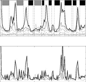
The next step is now to provide a “real space” description of the motions of the protein atoms, and examine how appropriate the models adopted by experimentalists are to describe such motions. In a typical experiment, it is not possible to label specific protons to monitor independently their motion. It follows that one probes the motion of all nonexchangeable protons (the protein is immersed in a D2O bath) simultaneously. Moreover, the structure factor is an intensive quantity representing scattering intensity per atom. Therefore, most if not all models used to describe the protein dynamics assume that mobile protons (those that give rise to a quasielastic signal in the time domain corresponding to the experimental resolution) have similar amplitudes and time scales of motion. The analysis of motion from MD simulations shows clearly that such models are inappropriate. Indeed, for proteins in solution, at room temperature, one finds that the protein motion is characterized by a very large heterogeneity. In particular, as shown in Fig. 23.7, the amplitudes of motion (mean-squared fluctuations) of di erent residues along the protein sequence can be as much as fiveto tenfold di erent. This is consistent with the sequence dependence of B-factors determined by X-ray crystallography [36] and previous analysis of MD simulations [37].

One interesting feature emerging from the simulation is the connection between the secondary structure and the amplitude of motions. Indeed, the results show that, as expected, the atoms belonging to those residues in highly structured regions of the protein (α-helices and β-sheets) are much less mobile that those attached to unstructured parts (e.g., loops) of the backbone, whether located at the surface of the protein or not. It is this kind of observation that should somehow be feed back into the experimental data analysis.

Inelastic neutron data are often interpreted in terms of a model of nonexchangeable hydrogen atoms di using in a sphere. The complexity of the models used to fit the data is limited by the small number of parameters that are extractable from the spectral lineshapes. Thus, it is important to keep in mind that, while the model of di usion-in-a-sphere fits QENS data reasonably well, it is clearly an approximation to ascribe a single sphere radius to hundreds or thousands of hydrogen atoms in a protein molecule.

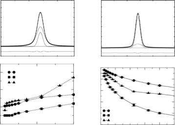
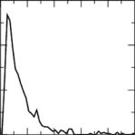
MD trajectories may be used to quantify the dispersion in the amplitudes of nonexchangeable hydrogen motion on the timescale probed by current neutron spectrometers. In Fig. 23.8 we show the distributions of the mean-squared fluctuations, ∆ri2 = (ri − ri2 )2 of the nonexchangeable hydrogen atoms in the MD simulations of the native α-lactalbumin in solution, computed as averages over blocks of 100 ps. The mean-squared fluctuations were calculated after removing the overall translational motion of the protein and hence represent the amplitudes of the internal motion. It is immediately evident that there is a broad distribution of H atom amplitudes on the 100 ps time scale. The distribution is sharply peaked at values near 0.5 ˚A, with pronounced asymmetry on the higher amplitude side.

To make contact with the di usion-in-a-sphere model we identify the average root-mean-squared fluctuation, ∆ri2 1/2, where the outer angular brackets denote an average over H atoms, with the average e ective radius of

go hand in hand, so that “raw data” may be compared side-by-side, and all the pitfalls, both in the simulation protocols and the experimental data analysis, may be identified and overcome.

Acknowledgment

This work has benefited from support from a collaborative grant between the University of Pennsylvania and the National Institute of Standards and Technology. We are grateful to Dr. Michael Klein for support and to Dr. Taner Yildirim for very helpful discussions and for providing software for scattering data analysis. This work was partially supported by a grant from the National Science Foundation (CHE-0417158).

References

1.W. Doster, S. Cusack, W. Petry, Nature 337, 754–756 (1989)

2.W. Doster, W. Petry, Phys. Rev. Lett. 65, 1080–1083 (1990)

3.Smith, J.C. Quart. Rev. Biophys. 24, 227–291 (1991)

4.C. Andreani, F. Menzinger A. Desidiri A. Deriu D. Di Cola, Biophys. J. 68, 2519–2523 (1995)

5.J. Fitter, R.E. Lechner, N.A. Dencher, Biophys. J. 73, 2126–2137 (1997)

6.G.R. Kneller, J.C. Smith, J. Mol. Biol. 242, 181–185 (1994)

7.J.M. Zanotti, S.H. Chen, Phys. Rev. E 59, 3084–3093 (1999)

8.A. Paciaroni, C. Arcangeli, A.R. Bizzarri et al., Eur. Biophys. J. 28, 447–456 (1999)

9.S. Timashe , in Stability of protein pharmaceuticals, Part B: In vivo pathways of degradation and strategies for protein stabilisation. (Plenum, New York, 1992)

10.M.J. Hageman, in Stability of protein pharmaceuticals, Part B: In vivo pathways of degradation and strategies for protein stabilisation. (Plenum, New York, 1992)

11.B. Hancock, G. Zografi, J. Pharm. Sci. 86, 1–12 (1997)

12.R.L. Remmele Jr., J.F. Carpenter, Pharm. Res. 14, 1548–1555 (1997)

13.M. Tarek, D.J. Tobias, J. Am. Chem. Soc. 121, 9740–9741 (1999)

14.M. Tarek, D.J. Tobias, J. Am. Chem. Soc. 102, 10450–10451 (2000)

15.M. Tarek, D.J. Tobias, Biophys. J. 79, 3244–3257 (2000)

16.M. Tarek, D.J. Tobias, J. Chem. Phys. 115, 1607–1612 (2001)

17.J. P´erez, J.M. Zanotti, D. Durand, Biophys. J. 77, 454–469 (1999)

18.Z. Bu, S-H. Lee, C.M. Brown, D.M. Engelman, C.C. Han, J. Mol. Biol. 301, 525–536 (2000)

19.Z. Bu, J. Cook, D.J.E. Callaway, J. Mol. Biol. 312, 865–873 (2001)

20.A. Gall, B. Robert, M.C. Bellissent-Funel, J. Phys. Chem. B. 106, 6303–6309 (2002)

21.A. Wlodawer, L. Sjolin, G. Gilliland, Biochemistry 27, 2705–2717, (1988)

22.J. Kuriyan, M. Karplus, G.A. Petsco, J. Mol. Biol. 192, 133 (1986)

23.J. Ren, K.R. Acharya, J. Biol. Chem. 266, 19292 (1993)

548M. Tarek et al.

24.M.C. Vaney, M. Riess-Kautt A. Ducruix, Acta. Cryst. D. Biol. Crystallogr. 52, 501 (1996)

25.M.P. Allen, D.J. Tildesley, Computer simulation of liquids (Clarendon Press, Oxford, 1989)

26.M.E. Tuckerman, G.J. Martyna, J. Phys. Chem. B 104, 159–178 (2000)

27.A.R. Leach, Molecular Modelling, Principles and Applications (Addison-Wesley Longman Limited; Singapore, 1996)

28.A.D. MacKerell Jr., M. Bellott, R.L. Dunbrack Jr. et al., J. Phys. Chem. B 102, 3586–3616 (1998)

29.U. Essmann, M.L. Berkowitz, T. Darden, L.G. Pedersen, J. Chem. Phys. 103, 8577–8593 (1995)

30.G.J. Martyna, M.L. Klein, J. Chem. Phys. 97, 2635–2643 (1992)

31.G.J. Martyna, M.L. Klein, J. Chem. Phys. 101, 4177–4189 (1994)

32.G.J. Martyna, D.J. Tobias, M.L. Klein, Mol. Phys. 87, 1117–1157 (1996)

33.J.-P. Ryckaert, H.J.C. Berendsen, J. Comp. Phys. 23, 327–341 (1977)

34.H.C. Andersen, J. Comp. Phys. 52, 24–34 (1983)

35.M. Be´e, Quasielastic neutron scattering: Principles and applications in solid state chemistry, biology, and materials science (Adam Hilger, Bristol, 1988)

36.E.D. Chrysina, K.R. Acharya, J. Biol. Chem. 47, 37021–37029 (2000)

37.E. Paci, C.M. Dobson, M. Karplus, J. Mol. Biol. 306, 329–347 (2001)

38.V. Receveur, J.C. Smith, M. Desmadril et al., Proteins: Struct. Funct. Genet. 28, 380–387 (1997)

39.D. Russo, J.M. Zanotti, M. Desmadril et al., Biophys. J. 83, 2792–2800 (2002)