306 COMPUTERS IN THE BIOMEDICAL LABORATORY

99.Fukunaga K, Hayes RR. Effects of sample size on classifier design. IEEE Trans Pattern Anal Machine Intell 1989;11: 873–885.

100.Sahiner B, et al. Feature selection and classifier performance in computer-aided diagnosis: the effect of finite sample size. Med Phys 2000;27:1509–1522.

101.Chan HP, Sahiner B, Wagner RF, Petrick N. Effects of sample size on classifier design for computer-aided diagnosis. Proc SPIE 1998;3338:846–858.

102.Chen DR, et al. Use of the bootstrap technique with small training sets for computer-aided diagnosis in breast ultrasound. Ultrasound Med Biol 2002;28:897–902.

103.Zheng B, Chang YH, Good WF, Gur D. Adequacy testing of training set sample sizes in the development of a computerassisted diagnosis scheme. Acad Radiol 1997;4: 497–502.

104.Tourassi GD, Floyd CE. The effect of data sampling on the performance evaluation of artificial neural networks in medical diagnosis. Med Decis Making 1997;17:186–192.

105.Efron B, Tibshirani RJ. An Introduction to the Bootstrap New York: Chapman and Hall; 1993.

106.Brem RF, et al. Improvement in sensitivity of screening mammography with computer-aided detection: a multiinstitutional trial. AJR 2003;181:687–693.

107.Burhenne LJW, et al. Potential contribution of computeraided detection to the sensitivity of screening mammography. Radiology 2000;215:554–562.

108.Moberg K, et al. Computed assisted detection of interval breast cancers. Eur J Radiol 2001;39:104–110.

109.te Brake GM, Karssemeijer N, Hendriks HCL. Automated detection of breast carcinomas not detected in a screening program. Radiology 1998;207:465–471.

110.Armato SG III, et al. Performance of automated CT nodule detection on missed cancers from a lung cancer screening program. Radiology 2002;225:685–692.

111.Getty DJ, Pickett RM, D’Orsi CJ, Swets JA. Enhanced interpretation of diagnostic images. Invest Radiol 1988;23:240–252.

112.Wu Y, et al. Artificial neural networks in mammography: Application to decision making in the diagnosis of breast cancer. Radiology 1993;187:81–87.

113.Jiang Y, et al. Improving breast cancer diagnosis with com- puter-aided diagnosis. Acad Radiol 1999;6:22–33.

114.Jiang Y, et al. Potential of computer-aided diagnosis to reduce variability in radiologists’ interpretations of mammograms depicting microcalcifications. Radiology 2001;220: 787–794.

115.Awai K, et al. Pulmonary nodules at chest CT: effect of computer-aided diagnosis on radiologists’ detection performance. Radiology 2004;230:347–352.

116.Brown MS, et al. Computer-aided lung nodule detection in CT: results of large-scale observer test. Acad Radiol 2005;12:681–686.

117.Chan HP, et al. Improvement of radiologists’ characterization of mammographic masses by using computer-aided diagnosis: an ROC study. Radiology 1999;212:817–827.

118.Fraioli F, et al. Evaluation of effectiveness of a computer system (CAD) in the identification of lung nodules with lowdose MSCT: scanning technique and preliminary results. Radiol Med (Torino) 2005;109:40–48.

119.Hadjiiski L, et al. Improvement in radiologists’ characterization of malignant and benign breast masses on serial mammograms with computer-aided diagnosis: an ROC study. Radiology 2004;233:255–265.

120.Huo Z, Giger ML, Vyborny CJ, Metz CE. Effectiveness of computer-aided diagnosis: Observer study with independent database of mammograms. Radiology 2002;224:560–568.

121.Kakeda S, et al. Improved detection of lung nodules on chest radiographs using a commercial computer-aided diagnosis system. AJR Am J Roentgenol 2004;182:505–510.

122.Kegelmeyer WP Jr, et al. Computer-aided mammographic screening for spiculated lesions. Radiology 1994;191:331–337.

123.Kobayashi T, et al. Effect of a computer-aided diagnosis scheme on radiologists’ performance in detection of lung nodules on radiographs. Radiology 1996;199:843–848.

124.Li F, et al. Radiologists’ performance for differentiating benign from malignant lung nodules on high-resolution CT using computer-estimated likelihood of malignancy. AJR Am J Roentgenol 2004;183:1209–1215.

125.MacMahon H, et al. Computer-aided diagnosis of pulmonary nodules: results of a large-scale observer test. Radiology 1999;213:723–726.

126.Shah SK, et al. Solitary pulmonary nodule diagnosis on CT: results of an observer study. Acad Radiol 2005;12:496–501.

127.Shiraishi J, Abe H, Engelmann R, Doi K. Effect of high sensitivity in a computerized scheme for detecting extremely subtle solitary pulmonary nodules in chest radiographs: observer performance study. Acad Radiol 2003;10:1302–1311.

128.Gur D, et al. Changes in breast cancer detection and mammography recall rates after the introduction of a computeraided detection system. JNCI 2004;96:185–190.

129.Feig SA, Sickles EA, Evans WP, Linver MN. Re: Changes in breast cancer detection and mammography recall rates after the introduction of a computer-aided detection system. JNCI 2004;96:1260–1261.

130.Paquerault S, et al. Improvement of computerized mass detection on mammograms: fusion of two-view information. Med Phys 2002;29:238–247.

131.Liu B, Metz CE, Jiang Y. An ROC comparison of four methods of combining information from multiple images of the same patient. Med Phys 2004;31:2552–2563.

132.Li Q, et al. Contralateral subtraction: a novel technique for detection of asymmetric abnormalities on digital chest radiographs. Med Phys 2000;27:47–55.

133.Schnall MD, et al. National digital mammography archive. In: Karellas A, Giger ML, editors. RSNA 2004 Categorical Course: Advances in Breast Imaging: Physics, Technology, and Clinical Applications. Oak Brook (IL): Radiological Society of North America; 2004.

134.Lloyd S, et al. Digital mammography: a world without film? Methods Inf Med 2005;44:168–171.

135.Cerello P, et al. GPCALMA: a Grid-based tool for mammographic screening. Methods Inf Med 2005;44:244–248.

136.Shah S, et al. Computer-aided diagnosis of the solitary pulmonary nodule. Acad Radiol 2005;12:570–575.

137.Aoyama M, et al. Automated computerized scheme for distinction between benign and malignant solitary pulmonary nodules on chest images. Med Phys 2002;29:701–708.

See also BIOTELEMETRY; COMPUTERS IN THE BIOMEDICAL LABORATORY;

MEDICAL EDUCATION, COMPUTERS IN; TELERADIOLOGY.

COMPUTERS IN CARDIOGRAPHY. See ELECTRO-

CARDIOGRAPHY, COMPUTERS IN.

COMPUTERS IN THE BIOMEDICAL

LABORATORY

GORDON SILVERMAN

Manhattan College

INTRODUCTION

Activities of daily living as well as within the industrial and scientific world have come to be domynated by machines

that are designed to reduce the expenditure of human effort and increase the efficiency with which tasks are completed. The technology underlying these devices is heavily dependent on computers that are designed for maximum flexibility, modularity, and ‘‘intelligence’’. A familiar example of flexibility comes to us from the automobile industry where a car manufacturer may use a single engine design for a large variety of models. These automobiles may also contain microcomputers that can sense and ‘‘interpret’’ road surfaces and adjust the car’s suspension system to maximize riding comfort. This type of design is characterized by the development of ‘‘functional’’ components that can be reused. The content of these elements, or ‘‘objects’’ as they are called, can be changed as technology improves, as long as access (or use) is not compromised by such changes. The characteristics of flexibility, modularity, and intelligence also exemplify instrumentation in the biomedical laboratory where, in recent years, laboratory sciences have become a matter of data and information processing. A user’s understanding of the tools of data handling is as much a part of the scientist’s skill set as performing a titration, conducting a clinical study, or simulating a biomedical model. Specific tasks in the biomedical (or other) laboratories have become highly automated through the use of intelligent instruments, robotics, and data processing systems. With the existence of >100 million internet-compatible computers throughout the world together with advanced software tools, the ability to conduct experiments ‘‘at-a-distance’’ opens such possibilities as remote control of such experiments and instruments, sharing of instruments among users, more efficient development of experiments, and report or publication of experimental data.

A new vocabulary has emerged to underscore the new computer-based biomedical laboratory environment. Terms such as bioinformatics (the scientific field that deals with the acquisition, storage, sharing and optimal use of information, data and knowledge) has come to characterize the biomedical laboratory culture. To understand contemporary biomedical laboratories and the role that the computer plays, it is necessary to consider a number of issues: the nature of data; how data is acquired; computer architectures; software formats; automation; and artificial intelligence.

Computers are instruments that process information, and within the biomedical laboratory they aid the analyst in recording, classifying, interpreting, and summarizing information. These outcomes encompass a number of specific instrument tasks:

Data handling: acquisition, compression, reduction, interpretation, and record keeping.

Control of laboratory instruments and utilities.

Procedure and experiment development.

Operator interface: control of the course of the experiment.

Report production.

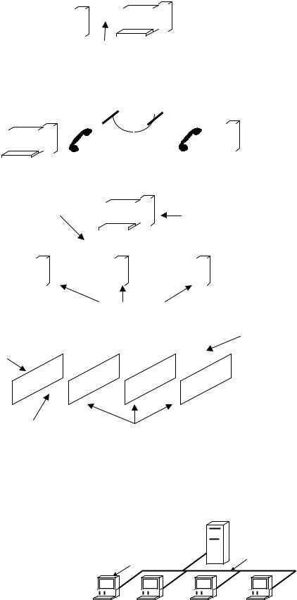
The biomedical laboratory environment is summarized in Fig. 1. Information produced by the experimental source

User information input

Figure 1. Information processing in laboratory environments.

may simply be recorded and the data analyzed at a later time. Alternatively, the data may be processed while the experiment proceeds and the results, possibly in reduced form, used to modify the experimental environment.

HISTORICAL ORIGINS

Scientific methodologies involving Biomedical laboratory research trace their origins to the experiments of Luigi Galvani in the 1789s with the study of ‘‘animal electricity’’

(1). This productive line of scientific investigation signals the start of the study of electrophysiology that continues to the present time. The ‘‘golden age’’ of electrophysiology began in the twentieth century (in particular starting 1920) and was led by such (Nobel recognized) scientists as Gasser, Adrian, Hodgkin, Huxley, Eccles, Erlanger, and Hartline, to name but a few (2). These scientists introduced the emerging vacuum tube technologies (e.g., triodes) to observe, record, and subsequently analyze the responses of individual nerve fibers in animal neural systems. The ingenious arrangements that the scientists used were based on an ‘‘analog computer’’ model. A sketch of such arrangements (3) for measuring action potentials is shown in Fig. 2. Of particular value was the cathode ray tube that could display the ‘‘rapid’’ electrochemical changes

Figure 2. Sketch of an early laboratory arrangement for measuring response of nervous tissue.

308 COMPUTERS IN THE BIOMEDICAL LABORATORY

from nervous tissue; this was a vast improvement over the string galvanometer that was previously used. A ‘‘highly automated’’ equivalent of this model with a digital computer architecture has been developed by Olansen et al. (4). Numerous electronic advances were made during the 1920s and 1930; Jan Toennies was one of the first bioengineers to design and build vacuum tube-based cathode followers and differential amplifiers. These advances found their way into the military technology of radar and other electronic devices of World War II. During the conflict, the electrophysiologists were pressed into service to develop the operational amplifier circuits that formed the basis of ‘‘computation’’ in the conduct of the war (e.g., firecontrol systems). While numerous advances in speed, and instrumental characteristics (e.g., increased input impedance, noise reduction) characterize wartime developments, equipment available in 1950 to continue electrophysiological work precluded rapid analysis of results; it took many weeks to calculate experimental results, a task that was limited to ‘‘pencil and paper’’ computations aided by electromechanical calculators. All this changed with the introduction of digital technology and the digital computer. H.K. Hartline was one of the first of the Nobel Laureates to automate the electrophysiological laboratory with the use of the digital computer. A highly schematic representation of Hartline’s experimental configuration is shown in Fig. 3 (5–7).

The architecture suggested in Fig. 3 became a fundamental model for information processing in the biomedical laboratory. However, within the digital computer, a number of (architectural) modifications have been introduced since the 1950s in order to improve informational throughput: the ability to complete data processing from acquisition to analysis to recording (as measured in ‘‘jobs/s’’).

DATA IN THE LABORATORY

An appreciation of the data underlying experiments in the biomedical laboratory is essential to successful implementation of a computer-based instrument system. The processing of experimental data is heavily dependent on the amount of information generated by the experimental preparation and the rate at which such data are to be processed by the computer. Both the quantity of data (e.g., the number of samples to be recorded) and the rate at which the data are to be processed can be estimated.

Figure 3. Early architecture of computer-automated biomedical laboratory environment. (After Hartline.)

These factors have important influence on the characteristics of the computer that is to be used in the design. A unit of information is the bit (as defined below), and the rate at which information is to be processed is determined by the capacity of the experimental environment (including any communications between the preparation and the rest of the system). The units of system capacity are bits/s. The following formulas are used to calculate these parameters:

P

InformationðbitsÞ ¼ H ¼ i pilog2ðpiÞ

Capacityðbits=sÞ ¼ C ¼ H=T

In these formulas, pi is the probability of experimental outcome i (the experiment may have a finite number of N outcomes) and log2 is the logarithm to the base 2. The ‘‘T’’ parameter is the time required to transmit the data from the preparation to the instrumental destination. (It must include any required processing time as well.) If all outcomes are equally likely (i.e., probable) then it can be readily shown that 2H ¼ N, where N is the total number of possible outcomes (and H is the information content in bits). The informational bit (H) is not to be confused with the term bit associated with binary digits. [Correlation of information (H) and the number of required binary processing digits may be correlated after appropriate coding.]

As an example of an appropriate calculation, consider one scientific temperature-measuring system that can report temperatures from 50 to 150 8C in increments of 0.01 8C. The system can thus produce 20,000 distinct results. If each of these outcomes is equally likely or probable, then the amount of information that must be processed amounts to 14.29 bits. Further, if the data processing system requires 0.1 s to generate a reading, then the capacity of the system is 142.9 bits/s. (As one cannot realistically subdivide a binary digit, 15 binary bits would be needed within the processing system.)

The formulas noted above do not describe the format of the data. For example, how many decimal places should be included. Generally, experiments are designed either to confirm or refute a theory, or to obtain the characteristics of a biological element (for purposes of this discussion). Within the laboratory there may be many variables that affect the data. In experimental environments, the results may often depend on two variables: one is the independent variable and the second, which is functionally related to the independent variable, is specified as the dependent variable. Other variables may act as parameters that are held constant for any given experimental epoch. Examples of independent variables include time, voltage, magnetizing current, light intensity, temperature, frequency (of the stimulating energy source), and chemical concentration. Dependent variables may also come from this list in addition to others.

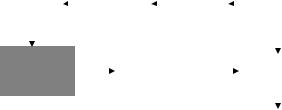
Two possibilities exist for the experimental variables: Their domains (values) may either be continuous or discrete (i.e., having a fixed number of decimal places) in nature. As a consequence, there are four possible combinations for the independent and dependent variables within the functional relationship; these are shown in Fig. 4, where the format ‘‘independent/dependent’’ applies to the axes. In Fig. 4, the solid lines represent actual values

Figure 4. Underlying information formats for biomedical laboratory data: (a) continuous–continuous; (b) continuous– discrete; (c) discrete–continuous; (d) discrete–discrete.

generated by the experimental preparation. The bold vertical lines emphasize the fact that measurements are taken only at discrete sampling times. ‘‘Staircase-like’’ responses indicate that only discrete values are possible for the dependent variable. Although any of the formats are theoretically possible, contaminants (noise for the dependent variable and bandwidth for the independent variable) usually limit the continuum of values. Thus, all instances of information in the biomedical laboratory are ultimately discrete–discrete (Fig. 4d) in nature. (In Figs. 4b–d, the dotted line reflects the original signal.)

The ability of a computer-based instrument system to discriminate between datum points is measured by its resolution and reflects the number of distinct values that a variable can assume. In the temperature-measuring example, there were 20,000 distinctly possible readings and consequently the resolution was 0.01 8C. When resolution is combined with the range of values that the variable can assume, the number of distinct experimental outcomes can be computed:

Number of unique experimental outcomes

¼ range=resolution

Summarizing the temperature-measuring system example in light of this relationship we conclude: resolution ¼ 0.01 (8C); range ¼ 200 (8C); number of outcomes ¼ 20,000. Within a computer-based data acquisition (DAQ) system, the values may appear as coded representations of the underlying outcomes. The codes might be related to the equivalent decimal values of the original data. However, one could also assign an arbitrary code to each outcome. Because computer-based systems are designed to interpret codes that have two distinct states (or symbols), binary coding systems are normally used in laboratory applications. A variety of binary coding schemes are possible. A simple, but effective, code employs the binary number system to represent experimental outcomes. A number in this system is a weighted combination of the two

symbols that are recognized in the binary number system, namely, 0 and 1. A complete representation of a binary number is given by

an2n þ an 12n 1 þ þ a121 þ a020 a 12 1 þ a 22 2 þ

where all coefficients (a values) are either 1 or 0. Starting with the least significant digit (20), the positional weights for the positive powers of 2 are 1, 2, 4, 8, 16, and so on. For the negative powers of 2, the weights in increasingly smaller values are 1/2, 1/4, 1/8, and so on. Table 1 contains a list of 16 possible outcomes from a (low resolution) laboratory experiment including both the binary and decimal equivalents. The outcomes might represent values of voltage, time, frequency, temperature, or other experimental variables.

The elements of a computer-based information processing system for biomedical laboratories are generally compatible with the binary system previously discussed. However, human users of such machines are accustomed to the decimal number system (as well as the alphanumeric characters of their native language). Within the system, internal operations are carried out using binary numbers and calculations. Binary results are often translated into decimal form before presentation to a user; numerical inputs, if in decimal format, are translated (by the computer) into binary format before use within the computer. Other number systems may be found in a computer application. These include octal systems (base 8) and the hexadecimal number system (base 16), where the base symbols include 0, 1,. . ., 9, A, B, C, D, E, F. A user may also be required to enter other forms of information such as characters that represent a series of instructions or a program. Several widely accepted codes exist for alphanumeric data, and some of these together with their characteristics are shown in Table 2.

Coded information such as that shown in Tables 1 and 2, may be passed (i.e., transmitted) between different elements of a computer-based laboratory information processing system. The communication literature provides a

rather complete description of the technology (8,9), and while it is not immediately germane to many circumstances of this discussion, some elements need to be mentioned. For example, the ‘‘internet’’ should be noted as an emerging development in computer-based biomedical laboratories.

There are two general protocols for transmitting laboratory data from the information source to its destination. Each part of the coded information (i.e., the bit) may be passed via a single communication channel. The channel element is the media and it might be wire, fiber optic cable, or air (as in wireless). Since there is only one channel, the data is passed in serial fashion, one bit at a time. An alternative arrangement permits the bits to be passed all at once (in parallel), but this requires an independent path for each bit such as a multiwire architecture. Parallel transmissions have inherently greater capacity than serial schemes. For example, if it requires 1 ms (i.e., 10 6 s) to transmit a bit, then a parallel transmission, using an 8-bit code, can pass 8 106 bits/s (i.e., 8 Mbits/s). An equivalent serial system would only have a capacity of 1 Mbit/s as it would require 8 ms for complete transmission of the code representing one of the possible experimental outcomes. Note that serial systems have a decided economic advantage over parallel schemes.

There are circumstances when two-way communication between elements of a computer-based data processing system is necessary. One element (e.g., the computer) may initiate a measurement instruction to a remotely located laboratory instrument (e.g., a spectrophotometer); the remote unit, in turn, responds with a set of measurements. Instructions, data, and parameters may need to pass from the computer, and status information (e.g., a busy signal) or results must be able to pass from the instrument to the computer: all of this over a serial path. Serial architectures can occur over a one-way (i.e., singlelane highway) or a two-way (i.e., two-lane highway) link. Figure 5 summarizes these communication alternatives.

In the half-duplex case, a single path must suffice for two-way communication. For proper transmission, the path must be made ready for communication in an appropriate direction before communication starts.

OVERALL ARCHITECTURE OF A COMPUTER-BASED BIOMEDICAL LABORATORY SYSTEM

The hardware for contemporary computer-based laboratory instrument systems reflects an information-processing model as shown in Fig. 1. A broad representative computerbased DAQ, and processing system is shown in Fig. 6. The

elements depicted in the figure can be divided into several categories: the computer [PC, laptop, personal digital assistant (PDA)], sensors (or transducers), signal conditioning components, DAQ, software, and other elements for other aspects of computer-based environments (remote instrumentation, external processors, vision/imaging equipment, and motion control apparatus).

Half-duplex

channel

Laboratory

instrument Computer

(a)

(b)

Figure 5. Serial communication alternatives: (a) half-duplex; (b) full-duplex.

Desktop

Sensors

Preparation, physical phenomena, or process

Figure 6. General arrangement of computer-based information processing system for biomedical laboratories.

The computer in such systems has considerable impact on the maximum throughput and, in particular, often limits the rate at which one can continuously acquire data. New bus (communication) facilities in the modern computer have greatly increased speed capabilities. A limiting factor for acquiring large amounts of data is often the hard drive (secondary storage system in the computer). Applications requiring ‘‘real-time’’ processing of high frequency signals often make use of an external (micro)processor to provide for preprocessing of data. (The term real-time refers to a guaranteed time to complete a series of calculations.) With the rapid development of new technologies, and the reduction is size, laptops and PDAs have found their way into the laboratory, particularly when the data is to be accumulated in isolated sites as with many biological experiments. With appropriate application software, laptops can act as data loggers [simple recorders of source (raw) data are collected] and further processing subsequently completed on a PC (or other) computer. Even greater miniaturization now permits PDAs to collect and transmit data as well. With wireless technology, data can be e-mailed to a base station. Also noted in Fig. 6 is the potential to connect the computer to a network [local area network (LAN), wide area network (WAN), or Internet] with the possibility of conducting experiments under remote control.

Sensors (see sensors) or transducers (10,11) sense physical phenomena and produce electrical signals that DAQ components can ultimately accept after suitable signal conditioning. Transducers are grouped according to the physical phenomena being measured. These devices have an upper operating frequency above which they produce a signal that is no longer independent of the frequency of the source (phenomena) frequency. Position is the most common measurement and sensors normally translate such physical distortions into changes in the electrical characteristics of the sensor component. For example, capacitive transducers rely on the fact that the capacitance depends on the separation (or overlap) of its plates. Since the separation is a nonlinear function of the separation, capacitive sensors are usually combined with a conditioning circuit that produces a linear relationship between the underlying phenomena and the potential delivered to the DAQ. Changes in the dimensions of a resistor alter its resistance. Thus, when a thin wire is stretched, its resistance changes. This can be used to measure small displacements and generate a measure of strain. Inductive principles are employed to measure velocity. When a mova-

ble core passes through the center of a coil of wire, the (electromagnetic) coupling is altered in a way that can be used to determine its velocity. Table 3 summarizes several applications.

Electrical signals generated by the sensors often need to be modified so that they are suitable for the DAQ circuitry. A number of conditioning functions are carried out in the signal conditioning system: amplification (to increase measurement resolution and compatibility with the full-scale characteristic of the DAQ); linearization (to compensate for nonlinearities in the transducer such as those of thermocouples); isolation (of the transducer from the remainder of the system to minimize the possibility of electric shock); filtering (to eliminate noise or unwanted interference such as those frequencies that are erroneous (e.g., high frequency or those from the power lines); excitation provides external signal source requirements for the transducer (such as strain gages that require a resistive arrangement for proper operation).

The DAQs normally include an analogue-to-digital converter (ADC) for converting analog (voltage) signals into a binary (digital) quantity that can be processed by the computer. There are several well-developed techniques for performing the conversion (12). As a general principle, the concept shown in Fig. 7 can be used to explain the conversion process.

Resistors in a high-tolerance network are switched in a predetermined manner resulting in an output voltage that is a function of the switch settings. This voltage is compared to the unknown signal and when this reference equals the unknown voltage the switch sequence is halted.

Figure 7. Principle of analog-to-digital conversion.

312 COMPUTERS IN THE BIOMEDICAL LABORATORY

The pattern of switches then represents a digital quantity equivalent to the unknown analogue signal. (Other schemes are possible.)

Several characteristics of the DAQ need to be considered when specifying this part of a computer-based processing system.

Range: The spread in the value of the measurand (experimental input) over which the instrument is designed to operate.

Sensitivity: The change in the DAQs output for a unit change in the input.

Linearity: The maximum percentage error between an assumed linear response and the actual nonlinear behavior. (The user should be assured that the DAQ has been calibrated against some recognized standard.)

Hysteresis: Repeatability when the unknown is first increased from a given value to the limit of the DAQ (range) and then decreased to the same (given) value.

Repeatability: Max difference of the DAQ reading when the same input is repeatedly applied (often expressed as a percentage of the DAQs range).

Accuracy: Maximum degree to which an output differs from the actual (true) input. This summarizes all errors previously noted.

Resolution: Smallest change in the input that can be observed.

Time Constant: Time required for the DAQ to reach 63.2% of its final value from the sudden application of the input signal.

Rise Time: time required to go from 5 to 95% of its final output value.

Response Time: time that the DAQ requires reaching 95% of its final value.

Settling Time: Time that the DAQ requires to attain and/or remain within a given range of its final value (e.g., 2% of its final value).

Delay Time: Time taken for the DAQ to reach 50% of its final value (not normally considered important).

Other sensor characteristics include: natural frequency, output impedance, mass, size, and cost.

Existing instruments may also be integrated into the computer-based environment if they include compatibility with a standard known variously as the General Purpose Interface Bus (GPIB) or IEEE 488: Originally developed by Hewlett-Packard (now Agilent) in 1965 to connect commercial instruments to computers (13). The high transfer rates (1MB/s) led to its popularity and it has evolved into an ANSI/IEEE Standard designated as 488.1, and subsequently as 488.2. The GPIB devices communicate with other such devices by sending device-dependent messages across the interface system (bus). These devices are classified as ‘‘Talkers’’, ‘‘Listeners’’, and/or ‘‘Controllers.’’ A Talker sends data messages to one or more Listeners that receive the data. The Controller manages the flow of information on the bus by sending commands to all devices. For example, a digital voltmeter has the potential to be a

Talker as well as Listener. The GPIB Controller is akin to the switching center of a telephone system. Such instruments may be connected to the computer system as seen in Fig. 6 as long as an appropriate component (card) is installed within the computer.

Images may be gathered from the biomedical laboratory using a (digital) camera and a suitable card within the computer. (See Olansen and Rosow in the Reading List.) Machine vision may be viewed as the acquisition and processing of images to identify or measure characteristics of objects. Successful implementation of a computer-based vision system requires a number of steps including:

Conditioning: Preparing the image environment including such parameters as light and motion.

Acquisition: Selecting image acquisition hardware (camera and lens) as well as software to be able to capture and display the image.

Analysis: Identification and interpretation of the image.

Computer-based (software) analysis of images takes into consideration the following:

Pattern Matching: Information about the presence or absence, number and location of objects (e.g., biological cells).

Positioning: Determining the position and orientation of a known object by locating features (e.g., a cell may have unique densities).

Inspection and Examination: Detecting flaws (e.g., cancer cells).

Gauging: Measuring lengths, diameters, angles and other critical dimensions. If the measurements fall outside a set of tolerance levels, then the object may be ‘‘discarded’’.

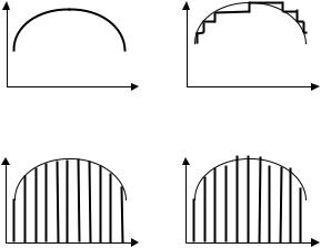
In addition to the acquisition of information from the laboratory, the computer system may be used to control a process such as an automated substance analysis using a robotic arm. (The motion control elements in Fig. 6 support such applications.) A sketch of such a system is shown in

Communication

(possibly lan) Sample rack

Scale Analytic

instrument

Figure 8. Computer-based architecture for an automated substance analysis system.

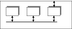
Fig. 8. The robotic arm would normally have several degrees of freedom (i.e., axes of motion) (14).

The system includes: a centrifuge (e.g., for analysis of blood samples); an analytic instrument (e.g., a spectrophotometer or chromatograph); a rack to hold the samples; a balance; a conditioning unit (possibly a stirrer or temperature oven); and instrumentation for dispensing, extracting and/or diluting chemicals. Various application programs within the computer could be used to precisely define the steps taken by the robotic arm to carry out a routine test. This program must also take into consideration the tasks to be carried out by each instrument (i.e., the drivers). When the computer does not obtain ongoing, continuous, status information from an instrument, the resultant arrangement is referred to as open-loop control of the particular instrument. In such cases, the program must provide for appropriate time delays (such as the time needed to position the robotic arm). Alternatively, the computer can receive signals from the various components that advise the program of their status; this is referred to as closed-loop control and is a generally more desirable mode of operation than the open-loop configuration.

COMPUTER BASICS

Personal computers are organized to carry out tedious, repetitive tasks in a rapid and error-free manner. The computer has four principal functional elements:

Central processing unit (CPU) for arithmetic and logical operations, and instruction control.

Memory for storage of data, results, and instructions (programs)

Input/output components (I/O) for interaction between the computer and the external environment.

Communication bus: or simply the bus, that allows the functional elements to communicate.

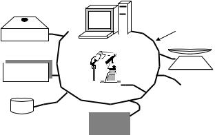
These elements are shown in Fig. 9 that comprises the functional architecture of the PC. Detailed descriptions, and operation of the PC and its components (e.g., secondary storage system—hard drive) are readily available (15). The architectures of computer-based instrument systems for laboratory environments generally fall into one of four categories; these are noted in Fig. 10.

A single-purpose (fully dedicated) instrument is shown in Fig. 10a. This arrangement is convenient because it is

External environment

Figure 9. Basic architecture of the PC.

consistent with such things as existing building wiring, particularly the telephone system although emerging developments also lend this architecture to a wireless arrangement. Standard communication protocols (previously noted) allow manufacturers to develop instruments to accepted standards. This arrangement may be limited to a single PC and a single instrument, and the distance between the host (PC) and the instrument may also be constrained. By adding additional communication lines, other instruments can be added to the single PC.

Remote control of instruments is depicted in Fig. 10b and is accomplished by adding devices within the PC that support communication over a traditional (standard) telephone line (including use of the internet). Real-time operation in such circumstances may be limited because time is required to complete the communications between the PC and the remote instrument placing significant limits on the ability of the system to obtain complete results in a prescribed time interval. Delays produced by the PCs operating system (OS) must also be factored into information processing tasks.

With the development of, and need for, instruments with greater capacity, new architectures emerged. One configuration is shown in Fig. 10c and includes a single PC together with multiple instruments coupled via a standard (i.e., IEEE 488) or proprietary (communication) bus. While such architectures are flexible and new instruments can be readily added, the speed of operation can deteriorate to the point where the capabilities of the PC are exceeded. Speed is reduced because of competition for (access to) PC resources (e.g., hard disk space).

The arrangement shown in Fig. 10d is referred to as ‘‘tightly coupled’’. In such cases, the instruments are integral to the PC itself. Communication between the PC and the instrument is rapid. Real-time (on-line) operation of the instrument is facilitated by a direct communication path (i.e., system bus) between the instrument and other critical parts of the PC such as its memory. No (external) PC controller is necessary and consequently the time delays associated with such functional elements do not exist. By varying the functional combinations, the system can be reconfigured for a new application. For example, functional components might include: data acquisition resources, specialized display facilities, and multiport memory for communication (message-passing) between the other elements.

Each of the arrangements in Fig. 10 includes a single PC. Additional operating speeds are possible (at relatively low cost) if more than one PC is included in the instrumental configuration. Such architectures are called multiprocessor-based instrument systems. Each processor carries out program instructions in its own right (16–18).

With the increasing complexity and capabilities of new software, a more efficient arrangement for computer-based laboratory systems has emerged. This is the client–server concept as shown in Fig. 11. The server provides services needed by several users (database storage, computation, administration, printing, etc.) while the client computer (the users) manage the individual laboratory applications (e.g., DAQ), or local needs (graphical interfaces, error checking, data formatting, queries, submissions, etc.).

Figure 10. Single-PC instrument architecture (a) Dedicated system. (b) One form of remotely controlled arrangement.

(c)Multiple instrument arrangement.

(d)Tightly coupled architecture.

SOFTWARE IN COMPUTER-BASED INSTRUMENT SYSTEMS

Programming consists of a detailed and explicit set of directions for accomplishing some purpose, the set being expressed in some ‘‘language’’ suitable for input to a computer. Within the computer, the components respond to two signals: þ5 V, or 0 V (ground). These potentials are interpreted as the equivalent of two logical conditions; normally the þ5 V is viewed to mean logically true (or logical 1), and a 0 V is interpreted as logically false (or logical 0). (Note that this is not universally true, and in

Server

Network

Client

Figure 11. The client–server architecture for biomedical laboratory environments.

some situations the logical 0 signals ‘‘true’’ while the logical 1 signals ‘‘false’’, but this is normally an exceptional case.) During the early 1950s, laboratory computers were programmed by entering a series of logical 1s and 0s directly into the computer using a series of switches on the computer’s front panel. A breakthrough occurred when English-like phrases could be used in place of these binary numbers. A series of programs within the machine called an assembler could be employed to interpret the instructions underlying the binary numbers. Within assembly language programs, English-like mnemonics are used in place of the numbers previously used to designate an instruction. The following example represents a series of assembly language instructions that might be used to add to quantities and store the results in one of the memory locations of the computer. (Text after the semicolon is considered to be a comment and not an instruction.)

During the 1950s, greater abstraction was introduced when text-based programming languages such as FORTRAN and COBOL were developed. Such languages are referred to as high level languages (HLLs). When individual versions are taken into account, there are literally hundreds of HLLs currently viable with languages such as C, Cþþ, and JAVA being prominent. By using HLLS, the three lines of code shown above could effectively be replaced by a single instruction:

C ¼ A þ B

Statements such as these made problem solving and programming more abstract, readable, and reduced the time it took to develop software applications. The statements are entered into the computer using a program called an editor; the code is then compiled and assembled (translated using a compiler program and an assembler program) to reduce the original text to the binary numbers needed to control the computer: the only ‘‘instructions’’ that a computer really ‘‘understands’’.

Rather than having to ‘‘rewrite’’ a program each time it was required, HLLs provided a means to develop highly abstract ‘‘application programs’’. A key development of such powerful resources was the introduction of Visicalc, the first (primitive) spreadsheet program: It is progenitor of such widely used programs as Excel, LOTUS, and others. Development of automated spreadsheet programs was motivated by the need for them in business applications, but they have come to find considerable utility in biomedical laboratory environments, particularly for data and statistical analysis as well as for data acquisition.

Increasing levels of abstraction in which programming details are hidden have continued to drive developments in software. A most important transition was made when software entered the age of ‘‘visual’’ programming. Arrangements and interconnections of functional icons have come to replace text when developing software for

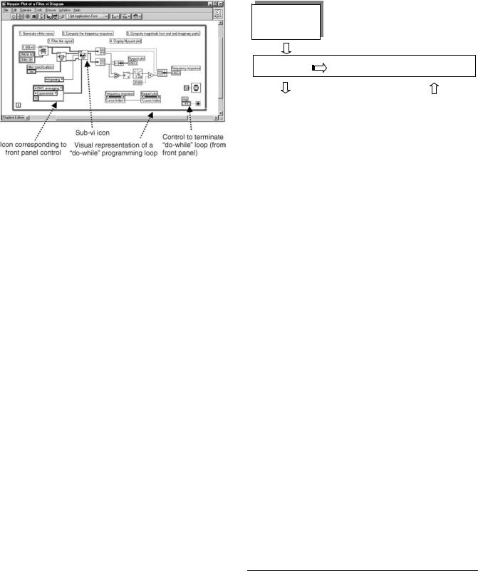
the biomedical laboratory. A key example of this architecture is the ‘‘graphic programming language’’ (GPL) called LabVIEW, which stands for Laboratory Virtual Instrument Electronic Workbench. This programming scheme provides work areas (windows) that the programmer uses to develop the software. In particular, the windows include a ‘‘Front Panel’’ and a ‘‘Diagram’’. This software enables a user to convert the computer into a software instrument that carries out real tasks (when coupled to appropriate elements as shown in Fig. 6). The Panel displays the indicators and controls that a user would find if the investigator had obtained a separate instrument for the experimental setup. Figures 12 and 13 are representative of a LabVIEW (front) panel and diagram. They are suitably annotated to indicate, controls, indicators, and symbols to replace traditional programming constructs (19).

The HLL programming is characterized by a control flow model in which the program elements execute one at a time in an order that is coded explicitly within the program. The narrative-like statements of the program describe the sequential execution of ‘‘Procedure A’’ followed by ‘‘Procedure B’’, and so on. In contrast, a visual programming paradigm functions as a dataflow computer language. This depends on data dependency; that is, the object in the block (node) will begin execution at the moment when all of its inputs are available. (This reflects a ‘‘parallel’’ execution scheme and is consistent with a multitasking model.) After completing its internal operations, the block will present processed results at its output terminals. While one node waits for events, other processes can execute. This is in

Figure 12. Front panel of a virtual instrument that obtains the attenuation and Nyquist characteristics (plot) of a filter that could be used in a Biomedical laboratory DAQ system. Control and display components are identified.

Figure 13. Diagram (Data Flow) of the virtual instrument for determining the frequency response and Nyquist plot of a filter.

some contrast to the control flow case where any waiting periods can create ‘‘dead time,’’ and may reduce the system throughput (20).

The virtual instrument (vi) depicted in Figs. 12 and 13 computes the frequency response of a digital filter and displays the attenuation versus frequency (the independent variable), as well as the imaginary part of the response versus the real part (i.e., Nyquist plot). In this example, a white noise signal is used as the stimulus of the filter and the vi returns the frequency response of the filter (21).

EMERGING AND FUTURE DEVELOPMENTS FOR COMPUTER-BASED SYSTEMS IN BIOMEDICAL LABORATORIES

Data processing in the biomedical laboratory is coming to rely increasingly on artificial intelligence (AI) for analysis, pattern recognition, and scientific conclusions. The development of ‘‘artificially intelligent’’ systems has been one of the most ambitious and controversial uses of computers in the biomedical laboratory. Historically, developments in this area (biomedical laboratory) were largely based in the United States (22–24). Artificial intelligent can support both the creation and use of scientific knowledge within the biomedical laboratory. Human cognition is underscored by a complex and interrelated set of phenomena. From one perspective, AI can be implemented with computer systems whose performance is, at some level, indistinguishable from those of human beings. At the extreme of this approach, AI would reside in ‘‘computer minds’’ such as robots or virtual worlds like the information space found in the Internet. Alternatively, AI can be viewed as a way to support scientists to make decisions in complex or difficult situations. For example, anesthesiology requires the health provider to monitor and control a great many parameters at the same time. In such circumstances, dangerous trends may be difficult for the anesthesiologist to detect in ‘‘real time;’’ AI can provide ‘‘intelligent control.’’ In science, AI systems have the capacity to learn, leading to the discovery of new phenomena and the creation of scientific knowledge. Modern computers and their associated appli-

Figure 14. Classification of artificial intelligence: Formal logic, Fuzzy Logic, Neural Nets.

cation software tools can be used to analyze large amounts of data, searching for complex patterns, and suggesting previously unexpected relationships (see Coiera in the Reading List). Simply stated, the goal of AI is to develop automata (machines) that function in the same way that a human would function in a given environment with a known complement of stimulants. In 1938, the British mathematician Alan Turing showed that a simple computational model (the Turing Machine) was capable of universal computation. This was one basis for the stored program model used extensively in modern computers.

An attempt to build an automaton that imitates human behavior falls into three broad categories: formal logic, ‘‘fuzzy’’ logic, and neural net technologies. These are depicted in Fig. 14.

While there is considerable overlap between human cognitive activities and machine technologies, in its most generic sense the relationships can be summarized in Table 4.

Historically, the first attempts at machine intelligence reflected formal logical thinking of which there are three kinds: deductive, inductive, and abductive. These are all built on a system of rules, some of which may be probabilistic in nature. Deductive reasoning is considered to be perfect logic : you cannot prove a false predicate to be true, or a true predicate to be true. The logic is built on the following sequence of predicates:

If p then q

p is true

Therefore q is true

By using the classification of beats in the ECG signal based on QRS duration and RR interval, we can develop a simple

Table 4. Human Cognitive Activities and Corresponding

Machine Technologies

example of deductive reasoning:

Allfbeats ðRR intervalÞ falling between 1:0 and 1:5s

having a QRS interval between 50 and 80 msgare normal

Patient’s f60th QRS complex occurs 1:25 s after the

59th complex with a duration of 60 msgPatient’s 60th

QRS complex is normal

Inductive conclusions, which can be imperfect and produce errors, follow from a series of observations. This logic is summarized by the following series of predicate statements:

From : ðP aÞ; ðP bÞ; ðP cÞ; . . .

Infer : ½forallðxÞðP xÞ&

(P a), (P b), (P c), and so on, all signify that entities whose properties are a, b, c, and so on, belong to the category identified as P. We therefore conclude that any object whose properties are similar to those of a, b, c, and so on, belong to the category identified as P. For example, a physician may observe many patients who have had fevers and some of who have subsequently died. Postmortem examination may reveal that they all had a lung infection (labeled ‘‘pneumonia’’). The physician may (erroneously) conclude that ‘‘all fevers must imply pneumonia’’, because he/she has a number of observations in which fever was associated with pneumonia.

Using cause–effect statements, abductive reasoning gather all possible observations (effects) and reaches conclusions regarding causes. For example, both pneumonia and septicaemia may both cause fever. The physician would then use additional observations (effects) to single out the ‘‘correct’’ cause. Abductive logic may also lead to false conclusions. Abductive logic follows from the argument that follows:

If p then q

q is true

Therefore p followsði:e:; is trueÞ

Using the circumstances just cited, a physician may (erroneously) conclude that having observed a fever, the patient is suffering from septicaemia. (It may, of course, also be due to pneumonia.)

Machine-Based Expert Systems

These systems require machine-based reasoning methods just noted and are depicted in Fig. 15. In addition, they must include stylized or abstracted versions of the world. Each of the representations in the database must be able to act as a substitute or surrogate for the underlying object (or idea). In addition, these tokens may have metaphysical features that reflect how the system intends to ‘‘think about the world’’. For example, in one type of representation known as a script, a number of predicates may appear that describe what is to be expected for a particular medical test. An Expert System for ‘‘detecting’’ an asystole in an ECG (electrocardiogram) might invoke the following rules (see Coiera in Further Reading):

Interface

User

Figure 15. Block diagram of a typical Expert System.

Rule 1:

If heart rate ¼ 0

Then conclude asystole

Rule 2:

If asystole andðblood pressure is pulsatile and in the normal rangeÞ

Then conclude retract asystole

Where knowledge is less certain, the rules might be modified. For example, for Rule 1, the conclusion might become,

‘‘conclude asystole with probability (0.8)’’.

A somewhat more informative example can be drawn from an interactive fragment from a contemporary medical Expert System (with similarities to the historical MYCIN software) (25):

The fragment does not represent a complete interactive session. The user would need to supply additional information to generate a potential diagnosis. An excellent demonstration of such systems can be found on the Internet:

http://dxplain.mgh.harvard.edu/dxp/dxp.sdemo.pl?/ login¼dems/cshome

While Expert System technologies have produced useful applications, they are confronted with a fundamental problem: How to determine what is ‘‘true’’ and what is ‘‘false’’. Contemporary systems address this in a variety of ways (e.g., providing a probabilistic result). This remains a problem for application software.

Fuzzy Logic Systems

These systems attempt to overcome the vagaries of truth and falsity and thus better reflect human thinking and may have some advantage over Expert Systems, where predicates are either true or false (or have some fixed probability of truth or falsity). Such systems were pioneered by Loti Zadeh in 1966 although exploitation began in earnest during the 1990s. [These are currently well over 2000 patents (many from Japan where this

technology was first embraced) and billions of dollars of sales of fuzzy products.] The concept underlying fuzzy logic is shown in Fig. 16 (26). Measurements in the real world are translated into equivalent linguistic concepts; the resulting ‘‘word’’ problems are solved in the linguistic world and conclusions are reconverted into physical entities that control elements in the real world.

Translation from physical measurements is accomplished by using a ‘‘belief system’’ (so called ‘‘membership functions’’) that reflects the degree to which we accept the particular measurement. A given measurement will then determine the extent to which we interpret its meaning. A representative set of membership functions is shown in Fig. 17, shown together with outcomes for a particular physical measurement (input).

A similar set of functions is also constructed to represent outputs, or rules, as summarized below. The output functions determine the extent to which we should set a particular control parameter in the physical system. In Fig. 17, we interpret the measurement to mean that we

have a 50% belief that it has a low value; we also believe that this measurement could represent a ‘‘medium’’ quantity, but we only have a 25% confidence in this value. (One might say, ‘‘The measurement is somewhere between a low and a medium value. Membership functions provides a measure of such informality.)

Degree of belief

Low value Medium value High value

Physical measure

Measurement

Figure 17. Fuzzy logic membership functions.

Figure 16. Paradigm for fuzzy logic control.

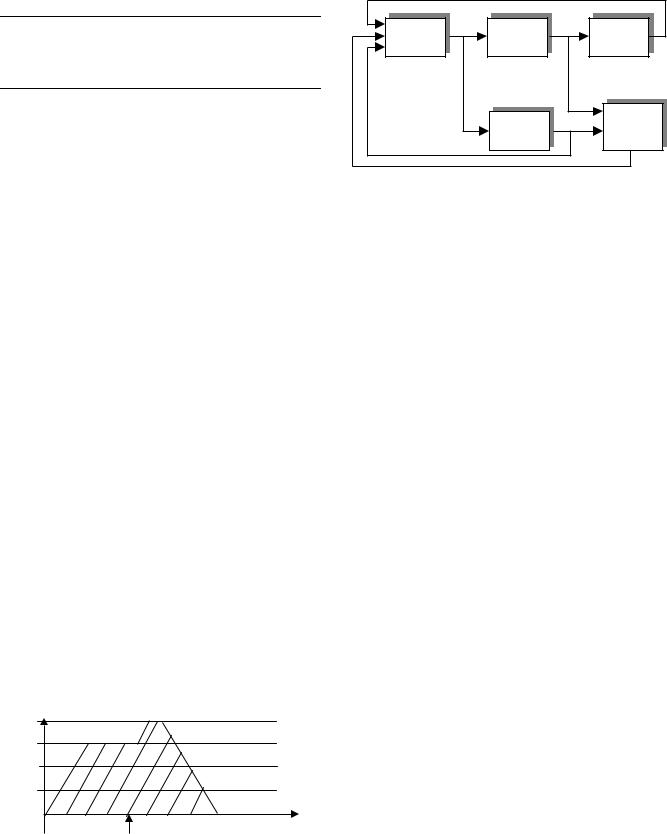
Table 5. Operations on Fuzzy Relations

aThe m stands for the membership or belief value as described in the narrative.

A system of rules also forms part of fuzzy control facilities. These rules have the following form:

If (physical parameter 1 is low) AND (physical parameter 2 is high) THEN (apply Rule 1 with a low intensity).

If (physical parameter 1 is medium) OR (physical parameter 2 is high) THEN (apply Rule 1 with a medium intensity)

The measurements and the logical operators (e.g., AND, OR, NOT) are employed according to the following set of (fuzzy) rules (as developed by Zadeh) (see Table 5).

For a given control problem, the measurement, application of the rules, and the invocation of actions leads to an overall profile of action; a typical result is shown in Fig. 18. From this a control value can be returned to the physical system: generating what is referred to as a crisp result (Defuzzification). There are several methods for obtaining this value from the curve noted in Fig. 18. Shown is the Center-of-Gravity method wherein the control value to be applied to the variable under control is the ‘‘balance point’’ of the curve.

Fuzzy control in a biomedical environment is exemplified by control of oxygen delivery to ventilated newborns in a neonatal intensive care environment (27). A sketch of the system is shown in Fig. 19.

For newborns requiring mechanical ventilation, oxygen toxicity is a potential danger that could result in chronic lung disease. Oxygen levels are also implicated in the development of retinopathy. Inspired oxygen concentration is commonly adjusted on an acute basis to control oxygen delivery and maintain patient saturation levels. The design of classic (engineering) control systems in such cases presents a significant challenge because of ‘‘transportation’’ delays. The alternative of manual control is also

Degree of belief

1.00

75

0.5

0.25

Output

Center of gravity

Figure 18. Defuzzification or generation of crisp results for a fuzzy logic control system.

Set point

Figure 19. Fuzzy control of inspired O2 concentration in ventilated infants.

unsatisfactory for two reasons: the patient might require increased O2 requirement but the manual increase is delayed due to delay in human response (e.g., the clinician is not present); the patient has decreased O2 requirement (clinical conditions improve) but the amount of O2 is not immediately decreased (because there is a perception that the patient is ‘‘doing well’’ and does not require intervention).

The Fuzzy model included some 35 rules, of which the following is one example:

If {change in oxygen saturation is small-negative} AND {rate of change in oxygen saturation is medium-negative}

THEN

{increase inspired oxygen concentration by a mediumpositive amount}

The membership curves for the various parameters will impose specific amounts for each rule that is invoked. Each rule yields an ‘‘action’’ value according to a membership class or extent to which the rule should be applied. A weighted mean of all rule outputs produces a single value for inspired oxygen concentration. This system maintained a target oxygen saturation (the set point determined by the health professional) better than routine manual control. It reduced overall oxygen exposure. No complex mathematical models were required as might be the case for traditional control with predictive capabilities. The rules are easy to understand and modify; expert knowledge about the problem was utilized. The controller was easily designed for nonlinear system responses: a goal that is daunting for traditional control technologies.

Neural Net (NN)

These systems employ a combination of circuits that approximate the behavior of neurological cells. While not limited to such applications, NNs are particularly useful for pattern recognition (28,29). Figure 20 shows the model of a single neuronal element and as well as a network of neuronal elements (NN).

The design of NNs is definitely not a precise enterprise; it is decidedly an art. A NN is ‘‘trained’’ to recognize patterns and while there are a great variety of NN

320 COMPUTERS IN THE BIOMEDICAL LABORATORY

Figure 20. Neural Net architecture. (a) A single neuron. (b) A NN showing input, hidden, and output layers with weighted interconnections.

architectures and training paradigms, a general scheme works as follows:

A NN is presented (at the input layer) with a set of ‘‘test’’ signals (e.g., samples of the input as a function of time). This is the so-called training set. If the NN produces an incorrect output (i.e., recognizing the wrong pattern), the weighted interconnections are automatically readjusted using an algorithm designated as back propagation (of error correction). The next time that the particular input sample is presented, the NN will tend to produce the correct answer.

Training continues until the NN satisfactorily recognizes the members of the training set. This recognition does not have to be perfect: just as human experts might disagree on the interpretation of a pattern.

The NN is then put into operation with inputs that it has not necessarily seen before; it will recognize whether or not the inputs have the same characteristics of the training set that it has been taught to recognize.

This process may be iterative; if the operational results are unsatisfactory, additional samples may be added to the training set and retraining instituted.

The NNs have been used to advantage in an ever-growing set of circumstances (30–32). In one instance, the NN (Hypernet) used a multi-layer architecture in which subjects’ anamnestic data, and 24-h diastolic and systolic blood pressure measurements were used as the parameters. System outputs included four 24-item arrays, whose values specify the hourly dosage to be administered to a patient for

each of the most common antihypertensive drugs. The presence and degree of hypertension (diagnosis) could be inferred from the drug dosage. No treatment was required for normal subjects whose records formed part of the training set. The system was evaluated on the basis of accuracy in both diagnosis and prescriptions. Hypernet correctly diagnosed 33 subjects out of 35, and 82% of the system’s prescribed treatment was deemed correct or acceptable by a group of medical experts.

SUMMARY

Biomedical laboratory instrument technology has changed markedly over the last 50 years. During the 1970s, a few daring scientific investigators began using the computer for instrument control and data acquisition. Such features are now commonplace add-ons to most instrumentation. The modern desktop computer system is a window into computing resources available anywhere in the world. Increasing levels of abstraction within the computer and its application software signal the emergence of a data processing model for experimental design within the Biomedical laboratory. This will only accelerate in the future as new computational algorithms are developed. Artificial intelligence as a knowledge-based tool is certain to grow manifestly in this emerging culture.

BIBLIOGRAPHY

1.Nebeker F. Golden accomplishments in Biomedical Engineering. Charting the milestones of Biomedical. Engineering. Engineering in Medicine and Biology Society; 2003.

2.Schoenfeld RL. From Einthoven’s Galvanometer to SingleChannel Recording. Charting the milestones of Biomedical Engineering, Engineering. Medicine and Biology Society; 2003.

3.Gasser HS, Erlanger J. A study of the active currents of nerve cells with the cathode ray oscilloscope. Am J Physiol 1922; 62: 406–524.

4.Olansen JB, Ghorbel F, Clark JW, Bidani A. Using virtual instrumentation to develop a modern biomedical engineering laboratory. Int J Eng Educ 2000; 16(3):244–254.

5.Schoenfeld RL. The role of a digital computer as a biological instrument. Ann New York Acad Sci 1964; 125(2):915–942.

6.Schoenfeld RL. How we know what the eye and the mind’s eye sees. IEEE Eng Med Biol Mag 1992; 11:47–71.

7.Silverman G, Eisenberg L. Programmable parallel timing system. IEEE Trans Biomed Eng 1971; 18(3):201–205.

8.Stallings W. Data and computer communications. 5th ed. New York: Prentice Hall; 1997.

9.Rappaport TS. Wireless communications; principles and practice. New York: Prentice Hall; 1999.

10.Carr JJ. Sensors and circuits. New York: Prentice Hall; 1993.

11.Norton HN. Handbook of transducers. New York: Prentice Hall; 1989.

12.Tyler M. The ABCs of ADCs. Scientific Computing & Instrumentation, April 2001; p 32–34.

13.Institute of Electrical and Electronics Engineers. IEEE Standard Digital Interface for Programmable Instrumentation, Standard IEEE 488.1, IEEE 488.2.

14.Liscouski J. Laboratory and scientific computing: A strategic approach. New York: John Wiley & Sons; 1995.