120COBALT-60 UNITS FOR RADIOTHERAPY

89.Lemke R, Klaus D, Lu¨ bbers DW, Oevermann G. Noninvasive ptCO2 initial slope index and invasive ptCO2 arterial index as diagnostic criterion of the state of peripheral circulation. Crit Care Med 1988;16:353–357.

90.Keller HP, Klaue P, Hockerts T, Lu¨ bbers DW. Transcutaneous pO2 measurement on skin transplants. In: Huch R, Huch A, Lucey JF, editors. Continuous Transcutaneous Blood Gas Monitoring, Birth Defects: Original Article Series. Volume XV-No. 4, New York: A.R.Liss; 1979.

91.Lu¨ bbers DW. Transcutaneous measurements of skin O2 supply and blood gases. Adv Exp Med Biol 1992;316:49–60.

92.Tremper KK, Waxman K, Shoemaker WC. Use of transcutaneous oxygen sensors to titrate PEEP. Ann Surg 1981;193:206–209.

93.Dooley J, Schirmer J, Slade B, Folden B. Use of transcutaneous pressure of oxygen in the evaluation of edematous wounds. Undersea Hyperb Med 1996;23:167–174.

94.Wattel F, Pellerin P, Mathieu D, Patenotre P, Coget JM, Schoofs M, Leps P. [Hyperbaric oxygen therapy in the treatment of wounds, in plastic and reconstructive surgery]. Ann Chir Plast Esthet 1990;35:141–146.

95.Huch A, Huch R, Hollmann G, Hockerts T, Keller HP, Seiler D, Sadzek J, Lu¨ bbers DW. Transcutaneous pO2 of volunteers during hyperbaric oxygenation. Biotelemetry 1977;4: 88–100.

96.Barker SJ, Tremper KK. The effect of carbon monoxide inhalation on pulse oximetry and transcutaneous pO2 [see comments]. Anesthesiology 1987;66:677–679.

97.Sridhar MK, Carter R, Moran F, Banham SW. Use of a combined oxygen and carbon dioxide transcutaneous electrode in the estimation of gas exchange during exercise. Thorax 1993;48:643–647.

98.Breuer HW, Skyschally A, Alf DF, Schulz R, Heusch G. Transcutaneous pCO2-monitoring for the evaluation of the anaerobic threshold. Comparison to lactate and ventilatory threshold [see comments]. Int J Sports Med 1993;14:417–421.

99.Sato M, Severinghaus JW, Powell FL, Xu FD, Spellman MJJ. Augmented hypoxic ventilatory response in men at altitude. J Appl Physiol 1992;73:101–107.

100.Alswang M, Friesen RH, Bangert P. Effect of preanesthetic medication on carbon dioxide tension in children with congenital heart disease. J Cardiothorac Vasc Anesthesiol 1994;8: 415–419.

101.Rozenfeld RA, Dishart MK, Tønnessen TI, Schlichtig R. Methods for detecting intestinal ischemic anaerobic metabolic acidosis by local pCO2. J Appl Physiol 1996;81:1834–1842.

102.Keller HP, Klaue P, Lu¨ bbers DW. Transcutaneous pO2 measurements on rats and rabbits. In: Huch R, Huch A, Lucey JR, editors. Continuous Transcutaneous Blood Gas Monitoring, Birth Defects: Original Article Series. Volume XV-No. 4, New York: A.R.Liss; 1979.

103.Tremper KK, Shoemaker WC. Continuous CPR monitoring with transcutaneous oxygen and carbon dioxide sensors. Crit Care Med 1981;9:417–418.

104.Versmold HT, Linderkamp O, Holzmann M, Strohhacker I, Riegel K. Transcutaneous monitoring of pO2 in newborn infants: where are the limits? Influence of blood pressure, blood volume, blood flow, viscosity, and acid base state. In: Huch R, Huch A, Lucey JF, editors. Continuous Transcutaneous Blood Gas Monitoring, in Original Article Series. Volume XV-No. 4, New York: A.R. Liss; 1979.

105.Wendling P, Fussinger R, Schmidt HD, Stosseck K. [Validity of the transcutaneous pO2-measurement during pharmacologically induced changes of skin perfusion (author’s transl)]. Anaesthesist 1982;31:135–138.

106.Ewald U, Huch A, Huch R, Rooth G. Skin reactive hyperemia recorded by a combined TcpO2 and laser Doppler sensor. Adv Exp Med Biol 1987;220:231–234.

107.Palmisano BW, Severinghaus JW. Transcutaneous pCO2 and pO2: a multicenter study of accuracy. J Clin Monit 1990;6: 189–195.

108.Tremper KK, Shoemaker WC. Transcutaneous oxygen monitoring of critically ill adults, with and without low flow shock. Crit Care Med 1981;9:706–709.

109.Fallenstein F, Ringer P, Huch R, Huch A. A new system for tcpO2 long-term monitoring using a two-electrode sensor with alternating heating. Adv Exp Med Biol 1987;220: 285–289.

110.Paky F, Koeck CM. Pulse oximetry in ventilated preterm newborns: reliability of detection of hyperoxaemia and hypoxaemia, and feasibility of alarm settings. Acta Paediatr 1995;84:613–616.

111.Baeckert P, Bucher HU, Fallenstein F, Fanconi S, Huch R, Duc G. Is pulse oximetry reliable in detecting hyperoxemia in the neonate?, Adv Exp Med Biol 1987;220:165–169.

112.Bragiroli A, Sacco C, Carone M, Donner CF. Pulse oximeter and transcutaneous O2 monitoring: criteria for a choice. Eur Respir J Suppl 1990;11:515s–517s.

113.Fallenstein F, Baeckert P, Huch R. Comparison of in-vivo response times between pulse oximetry and transcutaneous pO2 monitoring. Adv Exp Med Biol 1987;220:191–194.

114.Wimberley PD, Helledie NR, Friis-Hansen B, Fogh-Andersen N, Olesen H. Pulse oximetry versus transcutaneous pO2 in sick newborn infants. Scand J Clin Lab Invest Suppl 1987;188:19–25.

115.Wimberley PD. Oxygen monitoring in the newborn. Scand J Clin Lab Invest Suppl 1993;214:127–130.

116.Poets CF, Southall DP. Noninvasive monitoring of oxygenation in infants and children: practical considerations and areas of concern [see comments]. Pediatrics 1994;93:737–746.

117.Mike V, Krauss AN, Ross GS. Doctors and the health industry: a case study of transcutaneous oxygen monitoring in neonatal intensive care. Soc Sci Med 1996;42:1247–1258.

118.American Academy of Pediatrics Committee on Drugs: Guidelines for monitoring and management of pediatric patients during and after sedation for diagnostic and therapeutic procedures. Pediatrics 1992;89:1110–1115.

119.Wimberley PD, Burnett RW, Covington AK, Maas AHJ, Mueller-Plathe O, Siggaard-Andersen O, Weisberg HF, Zijlstra WG. Guidelines for transcutaneous pO2 and pCO2 measurement. IFCC document. Ann Biol Clin 1990;48:39–43.

See also BLOOD GAS MEASUREMENTS; CARDIOPULMONARY RESUSCITATION;

RESPIRATORY MECHANICS AND GAS EXCHANGE.

COBALT-60 UNITS FOR RADIOTHERAPY

JOHN R. CUNNINGHAM

Camrose, Alberta, Canada

INTRODUCTION

Cobalt is a metal, between iron and nickel, in the periodic table. It resembles them and occurs fairly commonly in iron and nickel ores, such as those found near Sudbury, Ontario, Canada. Cobalt as a substance has been known since about the mid-1700s. It was discovered in 1735 by a Swedish chemist named Brandt and was named after Kobald, a goblin from Germanic legends, known for stealing silver. Its salts were used in ancient days for making pigments, which produced brilliant blue colors in pottery.

The ancient Egyptians used it in painting murals in tombs and temples. It is necessary, in trace amounts, for proper nutritional balance.

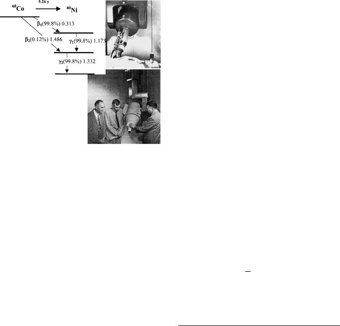
The nucleus of 59Co, which is the only isotope of cobalt found in Nature, has 27 protons and 32 neutrons. It happens to have an unusually large neutron capture crosssection, which means that bombardment with neutrons turns many of its atoms into 60Co, which is very highly radioactive. 60Co has a relatively long half-life (5.26 years) and it decays to 60Ni by the emission of a beta particle (an electron). 60Ni is also radioactive and emits two energetic gamma rays with energies 1.17 and 1.33 MeV. Million electron volts ¼ MeV. An electron volt is the amount of energy an electron has when it is accelerated through a voltage of 1 MV. It is very small: 1 MeV ¼ 1.602 10 13 J. These gammma-rays are produced in almost equal number and the pair of them can be approximated by their average 1.25 MeV, to form radiation that has high penetration in matter.

Cobalt has an atomic weight of 58.933 atomic mass units (amu), a mass density of 8900 kg/m3, and melts at 1500 8C. All of these properties combine to make it unique as a practical source of radiation for cancer treatment, industrial radiography, sterilization of food, and other purposes requiring intense but physically small sources of radiation.

It was not isolated as a metal until early in the eighteenth century and was not used for its metallic properties until the twentieth century. Its most important modern use is in the production of alloys of steel that are very hard and very resistant to high temperatures. These alloys find their uses in cutting tools and such diverse products as jet engines and kitchen cutlery.

HISTORY

Sampson et al. (1) noted the interesting radioactive properties of 60Co at least as early as 1936. Livingood and Seaborg

(2) described its properties in 1941. W.V. Mayneord, of the Royal Cancer Hospital in London (later the Royal Marsden Hospital), and A. J. Cipriani, then Head of the Biology Division at Chalk River, Ontario, Canada, described its production by neutron bombardment of 59Co in a nuclear reactor in 1947 (3).

In June of 1949, H.E. Johns, then professor of physics at the University of Saskatchewan, Canada, and physicist to the Saskatchewan Cancer Commission, visited the NRX nuclear reactor at Chalk River, Ontario, to discuss, with Cipriani and others, the possibilities of irradiating a sample of cobalt in order to produce a 60Co source. The theoretical advantages of using the energetic gamma rays of 60Co to destroy cancer cells had been known for some time, but practical problems of source production centered on the availability of a reactor with a sufficiently high neutron flux combined with a facility to handle and prepare the resulting highly radioactive source. Earlier, in 1945, J.S. Mitchell of Cambridge and J.V. Dunworth of Chalk River had discussed the possibilities of producing 60Co using the high neutron flux expected to be available from NRX, a nuclear reactor being built at the Chalk River site. At that time NRX was not yet operating, but in 1949, when

Johns visited it, it was. The NRX is a heavy water reactor and at that time had the highest available neutron flux in the world ( 3 1013 neutrons/cm2/s). The reactor was heavily involved in a program of radioisotope production and the irradiation of cobalt was taken to be part of this program.

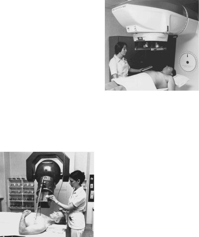
Arrangements were made to irradiate three samples of cobalt and they were placed in the reactor in the fall of 1949. They were removed 1.5 years later. The first source was destined for a cobalt unit being designed and built by Dr. Johns and his students in Saskatoon (4). It was delivered there in July of 1951 and on the 18th of August it was installed in the cobalt unit that had been prepared for it. The second source was sent to the Victoria Hospital in London, Ontario, where it was installed on the 23rd of October 1951 in a unit that had been designed and built by Eldorado Mining and Refining Company (later Atomic Energy of Canada Ltd.). Dr. Ivan Smith treated the first patient in London on 27th of October 1951, just 4 days after the installation of the source. The first patient treated on the Saskatoon unit, by Dr. T.A. Watson, was on the 8th of November 1951. Some mystery surrounds the details of the third source. There is some evidence that it was originally intended to go to Mayneord in England, but that in 1951 it was considered that postwar reconstruction was not yet sufficiently advanced there so it was diverted to the M.D. Anderson Hospital in Houston, Texas. It was to be installed in a unit designed by L.G. Grimmett, who had recently been hired by Dr. Gilbert Fletcher largely for this task (5). Part of the mystery concerns the fact that it was delayed in its irradiation and was actually removed from the reactor for a time and later replaced. Some have suggested that this may have been related to the outbreak of the Korean War and the general sensitivity concerning nuclear matters. Whatever the reason, it was not actually shipped until July of 1952, almost a full year later than the other two sources. The M.D. Anderson unit was then at Oak Ridge Tennessee for experimental purposes and was transferred, with its source, to the M.D. Anderson Hospital in Houston in September of 1953. The first patient was treated, in Houston, on the 22nd of February 1954. Pictures of these three cobalt units are given in Fig. 1. Roger F. Robinson has told an informative and interesting history, which includes many details about the original sources, as well as stories about a number of the people involved(6).

Each of these three sources was used in cobalt units for the treatment of cancer for many years. The two Canadian units became prototypes for units that were subsequently sold commercially. The unit in London, built by Atomic Energy of Canada Ltd., was the first of a long series of machines manufactured by them. The first series was known as the ‘‘Eldorado’’ series. A later series of units went under the name ‘‘ Theratron’’. The descendant of that company: MDS Nordion, is still building and selling cobalt units. The Saskatoon unit, designed by H. E. Johns and several of his students at the University of Saskatchewan, was made by John MacKay of the Acme Machine and Electric Co. Ltd. in Saskatoon (7) and later commercially by Picker X-ray of Cleveland, Ohio. Each of these units is pictured in Fig. 1 near the times of their source installations.

122 COBALT-60 UNITS FOR RADIOTHERAPY

Figure 1. The worlds first three cobalt units. Clockwise from above London, Ont., Canada, Saskatoon, Sask., Canada and Houston, Texas.

Before 1951, radiation therapy had been carried out almost exclusively by X-ray machines operating at tube voltages of 400,000 V or less. Such machines produce X-ray beams having a broad spectrum of X-ray energies with an average of one-third or less of the maximum. Thus, a 400 kV machine would correspond to a single energy of133 keV. Cobalt-60, with its average photon energy of 1.25 MeV, is the equivalent of an X-ray machine operating about six times the old value. As will be seen later, cobalt units are also mechanically and electrically simple devices and, following their introduction, rapidly became the standard machine for treating nearly all cancers other than that of the skin. Cobalt units have now been almost completely replaced by linear accelerators, which produce X rays having still greater penetration and higher outputs allowing shorter treatment times.

THE PHYSICS OF ACTIVATION: EXPOSURE AND DOSE

Only the physics directly related to the description of 60Co sources and units will be discussed here. More detailed information can be found in standard textbooks such as those of Attix (8), Greening (9), and Johns and Cunningham (10).

Almost any material placed within the neutron radiation field of a nuclear reactor will become radioactive. The probability of this happening is determined by the crosssection of the material for capturing a neutron. The crosssection is the equivalent of a probability, although it is usually expressed as an area. Many atoms have neutron capture cross-sections, of the order of 10 24 cm2 around 1935, Enrico Fermi, then in Rome, was measuring these cross-sections. When he found one of about this size he exclaimed, ‘‘ That’s as big as a barn!’’ 1 barn ¼ 10 24 cm2 is the common measure of nuclear cross-section and its use is permitted by the International System (SI) of units, and if a neutron passes through this area it is ‘‘captured’’ by the

Figure 2. The decay schemes of 60Co and 60Ni, showing the beta particle energies of 60Co and the gamma-ray energies from 60Ni.

nucleus to form a new nuclear species, which usually is radioactive.

The interaction of the neutron with a nucleus is quite complex, and a number of different products may be formed. The nucleus may capture the neutron to produce a new species that is stable, or the neutron may be re-emitted at the same or a different energy. In the latter case, we refer to the process as neutron scattering. The production of 60Co is an example of neutron capture. A nucleus of 59Co absorbs a neutron and forms 60Co, which is radioactive and decays with a half-life of 5.26 years by the emission of an electron that turns it into an isotope of nickel, 60Ni. The decay scheme of 60Co and 60Ni is shown in Fig. 2. The two gamma rays mentioned earlier are actually emitted by the Nickel nucleus 60Ni. Some properties of cobalt and its radiation are given in Table 1.

The 60Co activity produced is determined by the neutron flux density in the reactor, the neutron capture crosssection, the amount of 59Co inserted into the reactor, and the length of time it is left there. The rate of production of radioactive atoms can be expressed as

where N is the number of 59Co atoms placed in the reactor, s is the neutron capture cross-section per atom, f is the flux density of neutrons, and Dt is a time interval. The

Table 1. Properties of Cobalt and Its Radiation

parameter DN will be the number of activations that take place in this time interval.

As an illustrative numerical example, consider a sample of 15 g of 59Co to be located in a nuclear reactor at a point where

the neutron flux density is 1014 cm 2/s. This represents a source that is 1.5 cm in diameter and 1 cm high and is fairly representative of sources and neutron fluxes that have been used. The original two Canadian sources were 2.54 cm in diameter and composed of 26 disks each 0.5 mm thick. The American source was square in cross-section. From Eq. 1, and with the use of some of the information given in Table 1, we calculate the number of atoms of 59Co that are converted to 60Co during a period of time Dt. We also require a value for Avogadro’s Number NA, so that we can calculate the number of atoms (at) of 59Co in 1 g of the substance.

NA ¼ 6:023 1023 atoms=mol

The number of 59Co atoms in our 15 g sample is

From Table 1, we see that the cross-section for neutron capture in 59Co is 37 10 24 cm2/atom. If the 15 g of cobalt

were left in the reactor at this location for a period of 1 h, the number of atoms (at) converted to 60Co, following Eq. 1, would be

¼ 2:042 1018 at

Although this appears to be a very large number of atoms it represents only 0.2 mg of 60Co. It does, however, represent a considerable amount of radioactivity and would be easy to measure.

The most fundamental parameter for the specification of the strength of a radioactive source is activity. Activity is defined as the number of decay processes that occur per second and its special unit is the bequerel (Bq), which is defined to be an average of one nuclear disintegration each second. Activity is easy to describe theoretically, but is very difficult to determine experimentally. It can be inferred from the number of atoms of the substance and the value of its half-life, which for 60Co is given in Table 1 as 5.26 years.

Activity can be calculated from the simple relation

where l is a constant of proportionality known as the transformation constant. It is related to the half-life T1/2, of the radioactivity by

where the number 0.693 is the natural logarithm of 2. For example, the activity of 60Co that would result from

the above irradiation of 15 g of 59Co would be

where the half-life T1/2 has been expressed in seconds. The activity that is actually produced in a reactor irradiation is considerably less than this theoretical amount. This is largely due to attenuation of the neutron flux by the considerable mass of the cobalt.

The more traditional unit of activity has been the curie (Ci), which corresponds to 3.7 1010 nuclear decays/s. The activity of the above source, stated in curies would be

The specification of a commercial source of radiation in terms of activity is not very practical because activity does not uniquely relate to the radiation output when an individual source is loaded into a treatment unit. The output will depend on the physical size and configuration of the source and the design of the collimator of the treatment unit.

This problem was solved by the use of a quantity called exposure. Exposure is defined in terms of the amount of ionization that is produced in air by the radiation. The special unit is the roentgen (R). One roentgen corresponds to the release of 2.58 10 4 C/kg of air.

For gamma-ray emitters, such as this one, a quantity known as the exposure rate constant (G), has been defined that relates the activity in curies to the exposure rate in roentgen/hour at a point in air 1 m from the source. It is calculated from the gamma-ray spectrum using the interaction coefficients of air (the required data are given in Table 1). For a 60Co source, G, is

G ¼ 1:29 R m2=h Ci 1

This allows calculation of the parameter that is frequently used to specify source strength: the ‘‘roentgens per hour at a meter’’ (Rmm). For our 2.30 Ci source it is

A much more practical quantity, from the point of view of radiotherapy, is the absorbed dose rate produced at some agreed distance. To explain this, it will be useful to first define absorbed dose and to go through some approximate calculations connecting activity and absorbed dose rate.

Absorbed dose is the physical quantity that most closely correlates with the biological effect of the radiation and it is defined (11) as the amount of energy absorbed per unit mass of an irradiated material. The special unit of absorbed dose is the gray (Gy), which is defined as 1 joule (J) of energy imparted to 1 kg of matter.

A 60Co activity of 85.2 109 Bq, as derived above, would give rise to the following photon fluence rate at a distance of

The rate of photon interactions with a mass M of the water is given by

124 COBALT-60 UNITS FOR RADIOTHERAPY

where ci is the fluence (number crossing an area equal to 1 cm2) of each of the photon energies, (m/r)i is the mass interaction coefficient for each of them. The parameter(m/r) expresses the cross-section, or probability of interaction of photons with 1 g of material and M is the mass of the material in grams. The summation in Eq. 6 is over the two components of the photon spectrum as depicted in Fig. 2.

Since the photon energies are so close together, we can use the average value of the interaction coefficients, which is given in Table 1 as 0.0698 cm2/g. The rate of photon interactions, calculated from Eq. 6, would then be

Each photon that interacts imparts an average of 0.456 MeV (Table 1) of energy so the rate of energy absorbed E0, from this irradiation would be

This is a very tiny amount of energy. It was deposited in 1 g of water. Its value can be converted to a more familiar energy unit by using the relation 1 MeV ¼ 1.6022 10 13 J. The absorbed dose rate from these photons would then be

A simple radiation treatment for cancer typically involves an absorbed dose at the tumor of 2.0 Gy (in the old units; 200 rad), and because of attenuation in the tissues, and various other factors, this implies, for say a 2 min treatment, an activity almost 5000 times stronger than in our example source. The distance from the source to the tumor has typically been 80 cm. This would call for a source activity of 25 1013 Bq or 250 TBq or 7500 Ci.

To attain this, the cobalt must be left in the reactor for a much longer time than in our example above. With a longer activation, one must note that while 60Co is being formed it is also decaying. The resulting activity would be the sum of that which is being produced, as described by Eq. 1, and the amount that decays. This can

where N0 is the initial number of 59Co atoms present and l is the transformation constant (see Eq. 2) for the 6OCo decay. The other symbols have the same meaning as for Eq. 1. The solution to this equation, expressed in terms of activity, is

where Amax ¼ N0 s f is the maximum activity attainable for an infinitely long irradiation. For the neutron irradia-

tion conditions of our example, the maximum activity attainable is

It would require 5 years in the reactor to produce a source half this strong, that is, 7500 Ci.

This is not strong enough for modern treatment requirements and a higher neutron flux is required. As time has passed, reactor fluxes have increased considerably, and this has allowed both the irradiation times to be shortened and the sources to be made smaller.

There are a number of advantages to making cobalt sources as small as possible. One of these has to do with the sharpness of the edges of the radiation beam. This is known as penumbra and will be discussed later under that topic. It will be seen that a small diameter source is desirable. Another reason for a small source has to do with the amount of self-absorption and photon scattering that will take place within it. The source that we have been considering was a cylinder 1.0 cm in height, and for the gamma rays of cobalt this is almost a half value layer even in lead (Table 1), let alone in cobalt. It must be expected that the radiation emitted by such a source would be accompanied by considerable attenuation and would include an appreciable component of scattered photons. Because of the attenuation and scatter that takes place in the source, the dose rate is greatly overestimated in the calculations made above. The larger the source physically, the greater the activity required to give a desired dose rate.

SPECIFICATION OF SOURCE STRENGTH

In actual practice, the strength of the source is stated in terms of exposure rate at 1 m (Rmm). This is a measured quantity and is determined by the vendor of the source. Sources delivering up to 250 R/min at a meter are now available.

One way of judging the ‘‘efficiency’’ of the neutron irradiation is by stating the specific activity of the source produced. This is the activity, expressed in becquerel (or curie) per gram of cobalt. The specific activity of a 7500 Ci source that weighed 15 g would be 7500 Ci/15 g ¼ 500 Ci/g. In modern reactors, the neutron flux density can be greater than the 1014/cm 2 s 1 that we assumed, sources can be irradiated for longer times than in the example. Specific activities of up to 500 Ci/g have been produced. Cost goes up linearly with irradiation time, but, as can be seen, activity does not, and source strengths actually produced are decided by economic considerations. In actual practice, sources are not irradiated as solid cylinders, as has been assumed for this example, but rather they are made up into a capsule on demand from stocks or pellets that were preirradiated to a selection of specific activities. Pellets are shown in Fig. 3 along with a pair of stainless steel containers into which they will be placed. The pellets will be loaded into the cylinder shown in the center of the picture, then spacers, such as those shown on the right, are inserted to hold the pellets in position, and finally this cylinder, when capped, is inserted into the cylinder shown on the left and cold-welded shut. All

Figure 3. Cobalt pellets and source capsule with components.

of these operations are carried out remotely in a hot cell. Finally, the source is shipped in a well-protected and shielded container to be loaded into a cobalt unit.

COBALT UNIT DESIGN

The first cobalt units went into operation in 1951. Very soon after that they became available commercially, and the production of cobalt sources and cobalt units expanded to such an extent that, for 30 years, more radiotherapy was carried out with 60Co than with all other types of radiation combined. Cobalt machines have the tremendous advantages of producing a completely predictable, steady, reliable beam of relatively high energy radiation, being mechanically simple, rarely needing repair, and being easy to repair when required.

HEAD DESIGN

In all cobalt units, the source is placed near the center of a large, lead-filled steel container. A device is provided for moving the source from a position where it is ‘‘Off ’’, because it is shielded in all directions, to a position opposite an opening through which the useful beam may emerge. A number of mechanisms have been devised for moving the source, and two of them are shown in Fig. 4. In Fig. 4a, the source is mounted in a heavy metal (mostly tungsten) wheel that may be rotated through 1808 to carry it from the Off position to the On position. In Fig. 4b, the source is mounted in a sliding plug or drawer that carries it from the Off to the On position. In one of the first cobalt units (the Eldorado A), the source did not move at all. The beam opening was filled with a tank of mercury that was pumped out of the way by air pressure to turn the machine On and then the mercury returned by gravity to turn the beam Off.

Skin surface

Open

Closed

Figure 4. Two designs for cobalt unit heads. (a) A rotating wheel carries the source to the ‘‘on’’ position. A multiplane collimator controls the size of the rectangular beam. (b) A sliding drawer moves the source and a multileaf collimator moves on an arc to control the beam.

The sliding drawer mechanism shown in Fig. 4b has tended to be the more commonly used.

All machines must be arranged so that they fail ‘‘safe’’. That is, the source must be held in the On position by the continuous application of a force so that if the power fails, it must return quickly to the Off position. For both a and b in Fig. 4, this is provided by a strong spring. The lead-filled container, or ‘‘head’’ of the unit, must be of the order of 25 cm thick in all directions from the source. The design criteria will depend on the regulations in force where it is to be used, but basically it must be such that the leakage radiation emerging from the shield would not cause an overexposure to anyone staying at its surface for prolonged periods of time. This would imply, for example, a yearly equivalent dose of not > 5 mSv (or - 500 mrem) at a distance of 1 m from the source. This exposure level is greater than the average in low natural background areas, but is less than the exposure in many other regions of the world where people live. The sievert (Sv) is the special unit of equivalent dose. One sievert will result in the same biological effect as 1 (Gy) gray of conventional X rays. If we assume a maximum source strength of 10,000 Ci, and again use the exposure rate constant of 1.29 R m2/h Ci l, and assume that 1 R corresponds to an equivalent dose of 0.01 Sv, this would imply a thickness of 20–30 half-value layers. The half-value layer in lead for cobalt radiation is1.1 cm (Table 1), and this calculation would imply a thickness of 30 cm. In actual practice a much more detailed calculation would be done, augmented by measurement.

This simple calculation can serve as a guide only. The half-value layer for a broad beam of radiation, such as in

126 COBALT-60 UNITS FOR RADIOTHERAPY

this case, would be > 1.1 cm. On the other hand, it is unlikely that anyone would remain for a whole year just beside the head of the cobalt unit. In fact, 20–25 cm is about the thickness of the heads of most cobalt units.

Figure 4 also shows two types of collimators. Both consist of sets of bars that can be adjusted to produce a radiation beam with a rectangular cross-section. The diagrams at the bottom of Fig. 4 show an end-on view of the appearance of both collimator bars in the open and the closed positions.

MOUNTS

There are only two basic ways of mounting and ‘‘porting’’ radiation treatment units. One of the two oldest designs is illustrated in Fig. 5 and is an example of the so-called SSD mount. The head of the unit was held in a yoke, which was suspended by a column from a set of rails attached to the ceiling. It could be moved up and down or back and forth and the head could be rotated about the horizontal axis seen. The unit was also equipped with a treatment applicator, which in this case was mounted on the end of the collimator. The motions of the mount allowed the unit to ‘‘point’’ over a wide range of directions and enabled the operator to place the end of the treatment applicator against the skin of the patient at a prescribed location. The floor was left clear to allow easy and full movement of the treatment couch. The distance from the source to the skin of the patient (SSD) was thus a fixed quantity, usually 80 cm, and the focus of the ‘‘setup’’ was the surface of the patient. The size of the beam was defined there, and the reference point for dosimetry was just under the skin.

Figure 5. A Picker cobalt unit at the Ontario Cancer Institute, Toronto in the 1960s–1980s. The unit was mounted on a column suspended from rails on the ceiling leaving the floor clear. A protractor allows the angle to be set carefully using the ‘‘SSD’’ technique. The rack on the wall holds ‘‘wedge filters’’ that shape the beam intensity.

Figure 6. An isocentric mounted cobalt unit of the Theratron series produced by Atomic Energy of Canada Ltd., installed at the Ontario Cancer Institute in Toronto in the 1970s and 1980s.

The alternative mount is the so-called isocentric or fixed source-axis-distance (SAD) mount. An example, dating from the 1970s and 1980s is shown in Fig. 6. The head, encased in a streamlined plastic cover, is mounted on a gantry that can rotate about a horizontal axis. The patient lies on a couch as shown and is raised, lowered, moved sideways, or lengthways so that the tumor is positioned on the intersection of the gantry axis and the collimator axis. This means that for any angle of the gantry, the beam will pass through the tumor. This point is called the isocenter and was a fixed distance from the source, usually 80 cm, in later units 100 cm. The beam is specified by its size at the isocenter. The focus of attention is now at the tumor rather than the surface. In addition, the couch can usually be rotated about a vertical axis, also passing through the isocenter. Virtually all modern treatment units are mounted in the isocentric manner.

The procedures for treatment planning and dosimetry are somewhat different for each of these two types of mount. Treatment planning is discussed in several standard textbooks such as those by Bentel (12), Johns and Cunningham (10), and Kahn (13).

In 1956, an early and innovative symposium was held at Oak Ridge Institute of Nuclear Studies, just before the Eighth International Congress of Radiology, which was held in Mexico City. Problems of source production, machine design and installation, dosimetry, and source specification were discussed. The title of the publication that resulted from this symposium ‘‘Roentgens, rads and Riddles’’, largely reflected the uncertainties of the day in dosimetry. It also includes some history to that time and descriptions of a variety of cobalt units that had been made experimentally and by commercial suppliers.

Cobalt units are inherently simple machines and can be designed and constructed by relatively unsophisticated

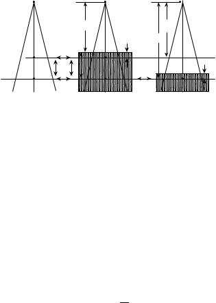
Figure 7. Three experimental cobalt unit designs: (a) a unit with a number of special features, (b) a double-headed unit, and (c) a unit for half-body irradiation.

engineering facilities. This is illustrated by Fig. 7, which shows three quite different units that were designed and built at the Ontario Cancer Institute in Toronto. The unit in (a) was built in 1959 and had a number of special experimental features (14). These included a diagnostic X-ray tube installed in the head of the unit so that good quality placement films could be taken of patients undergoing treatment. This facility is now standard equipment in all modern radiation treatment machines. The films are called ‘‘port films’’. It was isocentrically mounted and was capable of full 3608 rotation about the patient. This allowed continuous rotation during treatment or easy set up for the use of several fixed fields from different angles. The latter feature too, is standard on modern machines. The unit also had a large (95 cm) source-to-axis distance, which improved the depth dose characteristics (see the following section). This unit also had an ionization chamber in the counterweight so that the effective thickness of the patient could be determined. This did not prove to be as useful as expected and was not adopted by unit manufacturers.

The unit in Fig. 7b contained two sources and was called the Double-Header (15). The sources were arranged to be very nearly equal in strength and the beams were directed opposite to each other. This provided an automatic ‘‘parallel pair’’ of beams, which forms a component of many multiple field treatments. The real reason for the two sources, however, was to extend their useful life. The Ontario Cancer Institute had, at different times, as many as eight other cobalt units and two of the sources, after each had been used for 5 years (approximately one half-life) in

one or another of them were transferred to the DoubleHeader for another 5 years of use.

The third cobalt unit depicted in Fig. 7c, was especially designed for ‘‘half-body’’ treatments. It was equipped with a special collimator to provide radiation fields up to 150 cm long and 50 cm wide. It was fitted with a compensating filter so that a uniform dose distribution could be achieved (16).

CHARACTERISTICS OF THE RADIATION BEAM

The decay scheme for 60Co is shown in Fig. 2. There are two g rays of photon energies 1.17 and 1.33 MeV, respectively. These energies are very close to each other, so 60Co is almost a monoenergetic emitter with energy 1.25 MeV. The actual beam from a cobalt source also contains lower energy photons, which come from the scattering processes that take place within the source. It is also inevitably contaminated with photons scattered from the mechanism that holds the source in position as well as from the various collimator components that are ‘‘in view’’ of the source. That the beam is not purely that from 60Co is attested to by the fact that the linear attenuation coefficient for 1.25 MeV photons in water is 0.0698 cm l (Table 1), while the experimentally determined coefficient for a cobalt unit beam in water is closer to 0.063 cm l. A rather more ‘‘realistic’’ spectrum of the radiation for a cobalt unit has been determined by Rogers et al. (17) by Monte Carlo calculations. The low energy components contribute up to 15% to the dose received by the patient.

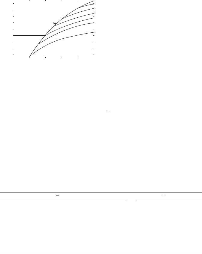
In a patient, the intensity of a radiation beam falls off approximately exponentially. This can be seen from the data plotted in Fig. 8, where percentage depth doses for cobalt-60 radiation, and a few other radiations used in radiotherapy, are shown plotted against depth. Percentage depth dose is the single most important quantity in choosing a radiation for radiotherapy. The radiations shown vary from that produced by 100 kV X rays to 25 MV. The depth at which the percentage depth dose falls to

Depth (cm)

Figure 8. Percentage depth doses plotted against depth for a series of beam energies from superficial (low energy X rays) to megavoltage radiation. All curves are for a 10 10 cm field and the depth to 50% dose can be easily determined.

128 COBALT-60 UNITS FOR RADIOTHERAPY

50% can be seen for each radiation by reference to the horizontal dashed line. It varies from < 2 cm for the superficial radiation through 7 cm for ‘‘conventional’’ or 250 kV radiation, 12 cm for 60Co radiation, to > 22 cm for the 26-MV radiation. Cobalt-60 is right in the middle of this range. The graphs in Fig. 8 also show that for the higher energies, the dose at the surface is low and rises as penetration increases. For 60Co radiation, it reaches its maximum at a depth of 0.5 cm and falls off relatively slowly from there. This low dose on the surface, the so-called skin sparing effect, was one of the important properties cobalt radiation had for radiotherapy.

When the cross-sectional area of a radiation beam is small, the dose received at a point below the surface is due almost entirely to primary radiation. As the area of the field is increased, the doses will increase due to an increase in scattered radiation. The greater the depth, the greater the increase, with the result that percentage depth dose increases with field size.

CALIBRATION

Calibration of the output of a cobalt unit is normally done with the use of an ionization chamber that has been calibrated against a standard exposure reference at a standardization laboratory. A calibration factor NX, is determined by the laboratory and its meaning is that NX ¼ X/M, where X is a known exposure and M is the reading of the electrometer monitoring the ionization produced in the chamber by the radiation.

The traditional and simplest method for calibrating the output of a cobalt unit has been to measure exposure rate in air at a chosen distance and field size, and to derive from this the absorbed dose rate that would occur at the center of a small mass of tissue-like material located at this point. An alternative, but equivalent, method is to determine the dose at a chosen position at a specified depth in a water phantom, again for a specified beam size.

Procedures for calibration, and the mathematical formalism required, to determine absorbed dose from exposure measurements are given in textbooks (9,10), as well as in various dosimetry protocols, both national and international. Examples are those of the American Association of Physicists in Medicine (18) and the International Atomic Energy Agency (19). Since the calibration procedures will only be outlined here, these sources should be consulted for more detailed procedures.

Calibration in Air

A number of physical arrangements for making measurements in a radiation beam are illustrated in Fig. 9. The diagram on the left can be used to refer to calibration in air. An ionization chamber, which has been calibrated in terms of exposure, is placed at point P0, free in air, and a reading, M, is taken for a specified ‘‘source-on’’ time T. This exposure time must be the actual exposure time; that is, it must be exclusive of a time, if any, taken for the source mechanism to move the source from the off to the on position. The reading, M, must also include any adjustment required for atmospheric conditions if the temperature and pressure

functions used for calibration and dose calculation for treatment planning.

differ from those that pertain to the exposure calibration factor. This would normally be 228C and 101.3 kPa (equivalent to 1 atm, or 760 mmHg). The parameter M must also be corrected for any small loss of charge that might occur due to charge recombination in the ion chamber during the exposure. Methods for making all of these corrections are discussed in Ref. 9,10,14, and 15. The ion chamber must also have been fitted with a buildup cap, if this is required to make its walls sufficiently thick to provide electronic equilibrium in them. The buildup cap must be made of water-like material. With these precautions, the exposure rate at the point designated in Fig. 9 as P0 would be

If the cobalt unit is ‘‘isocentric’’ in mount, point Q0 would be on the axis of rotation of the gantry, a distance FP from the source and the field size would be specified at this point. If the unit were operated in an SSD mode, the calibration point would be the one shown as Q0 in Fig. 9 and would be at a distance FQ from the source. The absorbed dose rate, free in air, may be calculated from the exposure by the following relationship:

air

The term in square brackets is derived from the definition of the roentgen, which is the release of a certain electrical charge per kilogram of air, and the average energy required to release 1 C of this charge. (One roentgen is defined as the release of 2.58 10 C/kg of air, and each coulomb released requires an average 33.85 J. Thus, 1 R corresponds to 0.00876 J/kg of air.) The next term is the ratio of mass energy absorption coefficients averaged over the radiation spectrum for water to air, and the final term is a correction factor to account for the fact that in order to characterize a dose rate at a point in air, it must be surrounded by at least enough phantom (water-like) material to produce electronic equilibrium. This material will attenuate and scatter radiations, and k(dQ), the allowance for this, is estimated to be 0.985.

Although the size of the beam at point P0 is larger than it is at point Q0, the collimator opening is the same for both,

Figure 10. Graphs showing relative output data for a cobalt unit. The output is measured in air and is expressed relative to that of a 10 10-cm field.

and so the source self-absorption and scatter, and collimator scatter, would be expected to be essentially the same. Consequently, the dose rate at P0 should be related to that at Q0 by the inverse square law. For any given cobalt unit this must be tested experimentally, but would be expected to be valid except for distances F, of Fig. 9, that are < 50 cm or so

On the other hand, if the collimator opening is changed, the dose rate at points such as P0 or Q0 will change, due principally to a change in the amount of collimator scatter reaching them. The way this output changes for an example cobalt unit is shown in Fig. 10, where relative dose rates measured on the axis (point P0 of Fig. 9) of an isocentric cobalt unit are plotted against the side length of a rectangular field. The data are normalized to 1.00 for a 10 10 cm field. From this diagram, it can be seen that

Table 2. Dosimetry Factors for 60Co Radiationa

ðmen=rÞwatmed

the dose rates differ by > 8% from a small, 5 5 cm field to a large 25 25 cm field. The family of curves shown represents rectangular fields, and it can be seen that a rectangular field gives approximately the same relative dose rate, as does a square field of the same area. For example, a 5 20 cm field shows a relative dose rate of almost exactly 1.00, as does the square field, 10 10 cm, of the same area. Curves such as these are specific to a particular collimator design and must be determined as part of the procedure of commissioning a new treatment unit.

Calibration in a Phantom

The right-hand diagram in Fig. 9 shows the arrangement for calibration in a phantom. The procedure is essentially the same as that for calibration in air; Q in this diagram has the same location and field size as does P0. The same precautions must be taken with the ion chamber reading and the same calibration factor, NX, is used. The dose rate at depth dQ in a water phantom is given by an expression that is very similar to that in Eq. 13:

ðmen=rÞairwat is, as before, the ratio of averaged mass-energy absorption coefficients, but in this case they should be

averaged over the photon spectrum that is present in the phantom. Values for this ratio are given in Table 2. It is generally assumed to be the same in the phantom as in air, although this cannot be quite correct, as shown by Cunningham et al. (20), Eq. 12. The factor k(c) is very similar to k(dQ) of Eq. 13, except that c is the radius of the ion chamber as it was configured when the calibration factor was obtained. This factor will be the same whether or not a buildup cap is actually in place in the phantom. The dose rate in a phantom, like that in air, varies with the field size, and a set of data like that shown in Fig. 10 can be compiled. The variation is greater, however, because the beam intensity incident on the phantom changes with collimator opening, as discussed previously, but in

ðmen=rÞmedair

130 COBALT-60 UNITS FOR RADIOTHERAPY

addition, the scatter generated within the phantom changes with a change in irradiated volume.

General Calibrations

Radiation beams of energy lower than that of 60Co are most frequently calibrated in air. Radiation beams higher in energy should always be calibrated in a phantom. Cobalt units, because of their energy and constancy of output, form a natural reference for all radiotherapy calibration procedures.

RELATIVE DOSE FUNCTIONS THAT ARE USED IN TREATMENT PLANNING

Over the years, a set of functions has been defined that make possible accurate point dose calculations as part of treatment planning. These are ‘‘tissue air ratio’’, ‘‘percentage depth dose’’, ‘‘backscatter factor’’, and ‘‘tissue phantom ratio’’. They are also used with radiations other than that from Co-60, but several of them were derived or refined for use with cobalt therapy. They will be discussed briefly. They can all be clarified by reference to Fig. 9.

Tissue Air Ratio (TAR)

Tissue air ratio, first called ‘‘tumor air ratio’’, was introduced by Johns to facilitate the calculation of tumor dose for rotation therapy. This type of treatment uses the isocentric mode of operation in that the tumor is placed on the axis of rotation of the treatment unit and the beam may be pointed toward the tumor from a selection of angles. The tissue air ratio, which may be defined by referring to Fig. 9, is the quotient formed by the dose, as determined for point P, on the central ray of the beam in a water phantom to the dose determined at the same point P0, with the water phantom removed. The dose at point P would be determined from Eq. 13 and the dose at P0 by Eq. 15, both exposures being made for the same time interval. In practice, it is assumed that all factors except the ion chamber readings will cancel, and tissue air ratios are actually taken to be

In this expression d, is the depth below the surface of the phantom and Wd is the field size at that depth. Tissue air ratio is an expression of the way the radiation beam is attenuated and scattered by the material of the phantom. It is the most fundamental of the relations discussed, and all of the others can be derived from it. Numerical data for this quantity for Co-60 are readily available.

Backscatter Factor

The ratio of doses determined from points Q and Q0 of Fig. 9 is a special value of the tissue air ratio. The depth, dQ, is the special depth just needed to produce electronic equilibrium at the point of dose measurement. At this point primary attenuation is the same in the phantom at Q and in the small mass of phantom-like material placed at Q0 in order to make the measurement. Most of the scattered radiation

reaching point Q is scattered backward from within the phantom. For the range of X rays that were in use before the advent of 6OCO, the depth dQ, was very small and the point Q, was considered to be on the surface, hence the name backscatter factor. This quantity is also called ‘‘peak scatter factor’’ because the depth at which electronic equilibrium is attained also tends to be the depth of peak dose in the phantom. For 60Co radiation, the depth of electronic equilibrium is taken to be 0.5 cm.

Percent Depth Dose

Whereas tissue air ratios relate doses in the phantom to doses free in air, percent depth doses interrelate doses at points within the phantom. Again referring to Fig. 9, the dose at point P is related to that at point Q by the percentage depth dose.

For this quantity, the field size is defined at the surface, and the distance F0 from the source to the surface must be stated. The doses at points P and Q should be determined from ion chamber measurements by the factors indicated in Eq. 15, and, as for tissue air ratios, it is generally assumed that all factors, except for instrument readings, cancel between the numerator and denominator.

Since point P is farther from the source than is Q, part of the falloff in dose with depth is due to the inverse square attenuation. Because of this, percentage depth doses increase with SSD. For example, the most common source–surface distance in use for Co-60 has been 80 cm. This was chosen as a compromise between increasing percentage depth dose and decreasing output. If the surface distance is increased from 80 cm to 1 m, the percentage depth dose at 10 cm in a 10 10 cm beam will increase from 55.6 to 57.8. This change is just slightly less than would be entirely accounted for by the inverse square law.

Tissue Phantom Ratios

For radiation of energy higher than that of cobalt, the dosimeter must be equipped with thick walls, and its size makes it inconvenient for use in air—particularly for small field sizes. It becomes convenient, therefore, to make the reference measurement in a phantom rather than in air. This is indicated in the right side of Fig. 9 by the point indicated by Q, which is the same distance from the source as is P (and P0), but is in a phantom at some chosen reference depth. The tissue phantom ratio is then the ratio DQ/DP and is entirely analogous to tissue air ratio and has many of the same properties. This quantity is, for example, also independent of distance from the source.

Tissue phantom ratios were introduced by Karzmark et al. (21) for use with high energy radiation, but can be applied equally well to Co-60 radiation.

Relationships between the Dose Calculation Functions

From Fig. 9, one can easily see the relationships between the various doses. For example, DP can be related to DQ directly by a percentage depth dose. It could also be

expressed by means of two tissue air ratios and the inverse square law:

The tissue phantom ratio is a combination of two tissue air ratios:

PENUMBRA

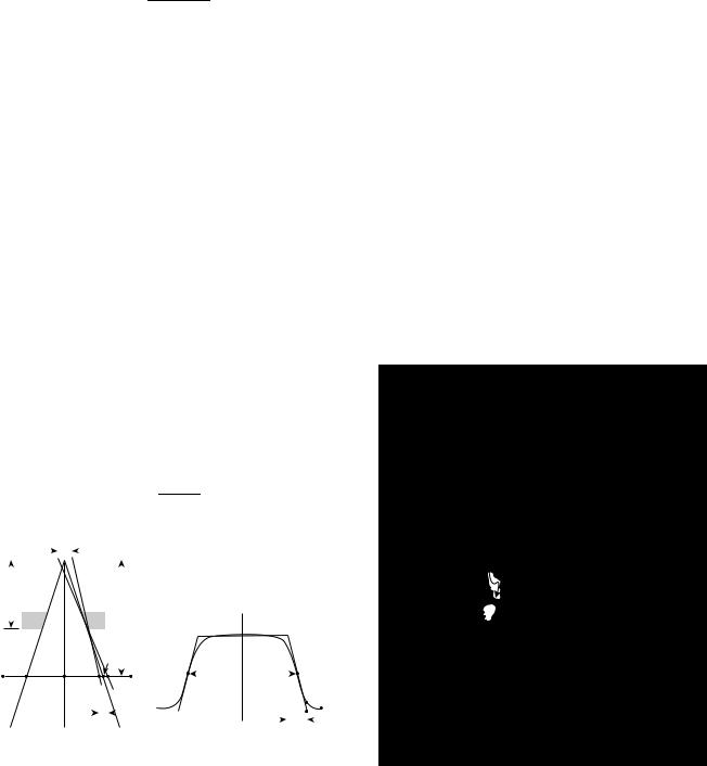
All of the previous considerations of dosimetry have been for points on the axis of the beam. Treatment planning is a 3D process, and regions not on the axis must also be considered. The behavior of the dose at points off the beam axis can be discussed by referring to Fig. 11.

In Fig. 11a, the radiation beam is incident on a point X0, in air. The conditions are the same as for the left side of Fig. 9. Consider a small dosimeter to be moved laterally across the beam from A to F. At A it is shielded by the collimator, while at X0 it is in the middle of the beam, in full ‘‘view’’ of the source. The dose will be at its greatest value at X0. At C it would still be in full view of the source, but it is slightly further away from the source than it is at X0 and the dose will be slightly lower. The expected doses at A, X0 and C, as well as other points on the line are shown by the dashed lines in Fig. 11b. At point D, the collimator blocks off half of the source and the dose would be expected to be one-half of its value at C. The point at E is just out of view of the source, and ideally the dose here should sink to zero. The portion of the line A–F between C and E is called the geometric penumbra. It is dependent on the diameter of the source, the distance fc, from the source to the end of the collimator, and the distance (f fc), from the end of the collimator to the line A–F. The geometrical penumbra is given by the very simple relation:

Figure 11. Diagrams showing the geometrical considerations involved in describing the shape of a cross-beam profile for a cobalt unit. (a) Shows the source and the collimator and (b) side shows a dose profile line A–F.

The actual measured penumbra differs somewhat from this and is always a little larger. The source does not behave like a sharp, well-defined disk because of its volume, and the radiation therefore scattered within it and the radiation scattered from the structures that hold it in place, and from the beam collimating apparatus. There is also, inevitably, some transmission through the collimator and some scattering from its lower end. The result is that the dose outside of the beam at points A and F is not zero, and the real dose profile is rounded off as depicted by the solid curve in Fig. 11b.

The shape of the dose profile in a phantom for 60Co radiation is only slightly different from that observed in air. The penumbral region is broadened somewhat by the transport of energy along the tracks of the electrons that are set into motion by the photons near the edge of the beam.

The meaning of field size can also be derived from Fig. 11. It is, by convention, taken to be the distance between points B and D. It is indicated as Wd in that diagram. This is the distance between the points that are at 50% of the dose on the axis at the same depth. It is also the full width at half maximum (fwhm) of the dose profile. Normally, the measurement of field size would be made in a phantom.

ISODOSE CHARTS

A more complete description of the dosage pattern of the beam is by means of an isodose chart. An isodose chart is a map of the distribution of the dose in a plane. Such charts are found in many books and papers in the literature and only one example will be given here. In Fig. 12, a small

80

S

Figure 12. Diagram showing an isodose chart for a beam from a cobalt unit treating a tumor in the neck of a patient. The target and some structures are shown.

132 COBALT-60 UNITS FOR RADIOTHERAPY

beam from an isocentric cobalt unit is treating a tumor in the neck region of a patient. This is an application for which cobalt radiation is still ideal. The target area, which is shown by the cross-hatched region, has been chosen by a radiation oncologist. A safety region has been allowed for and the beam is planned to be directed as shown. The dose at the target will be calculated from the calibration information as described above and (in this case) a tissue air ratio. On the diagram, it has been given the value 100. The solid lines in Fig. 12 show the distribution of percentages of the dose planned for the center of the target. In this case, the dose distribution has not been corrected for air cavities that might be in the path of the beam but modern treatment planning methods, carried out by computers, would include such considerations.

The dose at the center of the tumor is 77% of the maximum dose, and a single beam like this would not be deemed suitable. The planning process would be carried further by the addition of at least one more beam from another direction, so that the two would cross at the tumor and produce the maximum dose there. Such a treatment plan might even call for four or even more beams, all of which would be arranged to cross at the target.

Complete isodose distributions drawn for individually designed treatments for individual patients are part of the normal procedures of treatment planning. Dose calculation functions that have been discussed in this article have been incorporated into computer programs and enhanced into procedures that allow calculation of dose distributions for complicated treatment conditions. These calculation procedures have been refined to the extent that the 3D shape of the patient and tissue inhomogeneities can be accounted for. The development of these calculation methods has a lengthy history. Suffice it to say that current methods of calculation use Monte Carlo procedures and are quite precise.

NOTABLE FIRST CLINICAL APPLICATIONS

The use of large irregularly shaped radiation beams was introduced for use with cobalt units in the late 1950s. The task was irradiation of chains of lymph nodes for treatment of Hodgkin’s disease. This was so successful that a diagnosis of this disease went from a virtual ‘‘death sentence’’ to one that was highly curable. These ‘‘mantle’’ fields, frequently shaped from low melting point lead alloys for individual patients, are still in use. One of the earliest developments of a computer program for the calculation of the dose distribution was introduced with these treatments in mind (22). This program too, is still in use.

A precursor to today’s intensity modulation radiation therapy was instituted in the 1960s in Japan by Takahashi who described the use of multileaf collimators and dynamic treatment delivery with a cobalt unit in 1963 (23).

A group under A. Green at the Royal Northern Hospital in London, England pioneered conformal radiation therapy by developing cobalt machines in which the patient was automatically positioned during rotational therapy by moving the treatment couch and machine gantry by electromechanical systems. It was given the name ‘‘The

Tracking Cobalt Project’’ because it attempted to make the dose distribution conform to the spread of the disease. With a similar intent Proimos in Patras, Greece and later Rawlinson and Cunningham in Toronto (24), described the use of synchronous shielding in a Co-60 beam to make the radiation beam conform to the target while avoiding critical normal tissues.

SUMMARY AND CONCLUSIONS

It is still likely, even now, that more cancer patients have been treated by radiation from cobalt units than by any other kind of radiation. The number is estimated to be > 30 million (25). The cobalt unit was the backbone of radiation therapy for over four decades. The cobalt unit is mechanically simple and its output is totally predictable and reliable. Sources with sufficient strength to enable practical, short treatment times can easily be produced. Because of the source decay, sources must be renewed at intervals of 5 years or so, but this procedure is quite straightforward and its expense is more than offset by the low maintenance cost of the machine.

The beam characteristics are well known and relatively easy to measure. It is also easy to make special filters and beam modifiers for individual treatment needs. The energy is high enough to provide skin sparing. The most important single parameter in choosing a radiation energy for therapy is depth dose and the depth dose of cobalt radiation is quite satisfactory for treating tumors that are within 10 cm or so of the surface. This includes head and neck tumors and all but deep-seated lesions in very large patients. With respect to this quantity 60Co is in the middle ground. It remains the unit of choice as a first unit in a developing department and is a must as part of the equipment for any large radiotherapy department. Cobalt units are still being manufactured and sold at about half the rate that obtained at the peak of their use. Modern cobalt units include many of the technological innovations, such as computer control, that are part of the more modern treatment machines. An excellent chapter on Co-60 and its role in modern times has been written by Glenn Glasgow (26). This is recommended to the interested reader.

BIBLIOGRAPHY

1.Sampson M, Ridenouri LN, Bleakney W. A long lived radiocobalt produced by irradiating cobalt with neutrons. Phys Rev 1936;50:382.

2.Livingood JJ, Seaborg GT. Radio-active isotopes of Cobalt. Phys Rev 1941;60:913.

3.Mayneord WV, Cipriani AJ. The absorption of gamma-rays from 60Co. Can J Res Sec A: Phys Sci 1947;25:303.

4.Johns HE, Bates LM, Watson TE. 1000 curie cobalt units for radiation therapy. The Saskatchewan cobalt-60 unit. Br J Radiol, 1952;25:296.

5.Grimmett LG, Kerman HD, Brucer M, Fletcher GH, Richardson JE. Design and construction of a multicurie cobalt teletherapy unit. A preliminary report. Radiology (Easton Pa) 1952;59:19.

6.Robinson RF. The race for Megavoltage. Acta Oncol 1995; 34:1055.