

- •VOLUME 2
- •CONTRIBUTOR LIST
- •PREFACE
- •LIST OF ARTICLES
- •ABBREVIATIONS AND ACRONYMS
- •CONVERSION FACTORS AND UNIT SYMBOLS
- •CARBON.
- •CARDIAC CATHETERIZATION.
- •CARDIAC LIFE SUPPORT.
- •CARDIAC OUTPUT, FICK TECHNIQUE FOR
- •CARDIAC OUTPUT, INDICATOR DILUTION MEASUREMENT OF
- •CARDIAC PACEMAKER.
- •CARDIAC OUTPUT, THERMODILUTION MEASUREMENT OF
- •CARDIOPULMONARY BYPASS.
- •CARDIOPULMONARY RESUSCITATION
- •CARTILAGE AND MENISCUS, PROPERTIES OF
- •CATARACT EXTRACTION.
- •CELL COUNTER, BLOOD
- •CELLULAR IMAGING
- •CEREBROSPINAL FLUID.
- •CHEMICAL ANALYZERS.
- •CHEMICAL SHIFT IMAGING.
- •CHROMATOGRAPHY
- •CO2 ELECTRODES
- •COBALT-60 UNITS FOR RADIOTHERAPY
- •COCHLEAR PROSTHESES
- •CODES AND REGULATIONS: MEDICAL DEVICES
- •CODES AND REGULATIONS: RADIATION
- •COGNITIVE REHABILITATION.
- •COLORIMETRY
- •COMPUTERS IN CARDIOGRAPHY.
- •COLPOSCOPY
- •COMMUNICATION AIDS FOR THE BLIND.
- •COMMUNICATION DEVICES
- •COMMUNICATION DISORDERS, COMPUTER APPLICATIONS FOR
- •COMPOSITES, RESIN-BASED.
- •COMPUTED RADIOGRAPHY.
- •COMPUTED TOMOGRAPHY
- •COMPUTED TOMOGRAPHY SCREENING
- •COMPUTED TOMOGRAPHY SIMULATOR
- •COMPUTED TOMOGRAPHY, SINGLE PHOTON EMISSION
- •COMPUTER-ASSISTED DETECTION AND DIAGNOSIS
- •COMPUTERS IN CARDIOGRAPHY.
- •COMPUTERS IN THE BIOMEDICAL LABORATORY
- •COMPUTERS IN MEDICAL EDUCATION.
- •COMPUTERS IN MEDICAL RECORDS.
- •COMPUTERS IN NUCLEAR MEDICINE.
- •CONFOCAL MICROSCOPY.
- •CONFORMAL RADIOTHERAPY.
- •CONTACT LENSES
- •CONTINUOUS POSITIVE AIRWAY PRESSURE
- •CONTRACEPTIVE DEVICES
- •CORONARY ANGIOPLASTY AND GUIDEWIRE DIAGNOSTICS
- •CRYOSURGERY
- •CRYOTHERAPY.
- •CT SCAN.
- •CUTANEOUS BLOOD FLOW, DOPPLER MEASUREMENT OF
- •CYSTIC FIBROSIS SWEAT TEST
- •CYTOLOGY, AUTOMATED
- •DECAY, RADIOACTIVE.
- •DECOMPRESSION SICKNESS, TREATMENT.
- •DEFIBRILLATORS
- •DENTISTRY, BIOMATERIALS FOR.
- •DIATHERMY, SURGICAL.
- •DIFFERENTIAL COUNTS, AUTOMATED
- •DIFFERENTIAL TRANSFORMERS.
- •DIGITAL ANGIOGRAPHY
- •DIVING PHYSIOLOGY.
- •DNA SEQUENCING
- •DOPPLER ECHOCARDIOGRAPHY.
- •DOPPLER ULTRASOUND.
- •DOPPLER VELOCIMETRY.
- •DOSIMETRY, RADIOPHARMACEUTICAL.
- •DRUG DELIVERY SYSTEMS
- •DRUG INFUSION SYSTEMS
284 COMPUTER-ASSISTED DETECTION AND DIAGNOSIS
King MA, Tsui BM, Pan TS, Glick SJ, Soares EJ. Attenuation compensation for cardiac single-photon emission computed tomographic imaging: Part 1. Attenuation compensation algorithms. J Nucl Cardiol 1996; 3:55–64.
Groch MW, Erwin WD. SPECT in the year 2000: basic principles. J Nucl Med Technol 2000; 28:233–244.
Cherry SR, Sorenson JA, Phelps ME. Physics in Nuclear Medicine. 3rd ed. Philadelphia: Saunders: 2003. p 299–324.
See also ANGER CAMERA; NUCLEAR MEDICINE INSTRUMENTATION; POSITRON EMISSION TOMOGRAPHY; RADIOPHARMACEUTICAL DOSIMETRY.
COMPUTER-AIDED RADIATION DOSE
PLANNING. See RADIATION DOSE PLANNING, COMPUTER-
AIDED.
COMPUTER-ASSISTED DETECTION
AND DIAGNOSIS
ROBERT M. NISHIKAWA
The University of Chicago
Chicago, Illinois
INTRODUCTION
Since their discovery, X rays have been used to make images (radiographs) that allow the internal condition of the human body to be examined. Reading or interpreting these images has been without exception performed solely by humans until very recently. As our society depends more and more on automation or assistance from automated systems, so too has the interpretation of radiographs, although still in a very limited way at the present time.
In the early 1960s, researchers attempted to automate the interpretation of radiographs. The first published study was by Winsberg et al. who developed an automated computerized scheme to diagnosis breast cancer from a radiograph of the breast (mammogram) (1). This attempt, like others from that time period, was largely unsuccessful. Compared to current technology, these studies suffered from poor quality film digitizers (all images were recorded on film), insufficiently powered computers that had severely limited memory and storage space, and only a rudimentary armament of image processing, pattern recognition and artificial intelligence techniques. Clearly, the goal of automating the interpretation of radiographs was beyond the technical capabilities of that era.
After those initial attempts, there was a period of inactivity. In the late 1980s, a new approach was developed called computer-aided diagnosis (CAD) (2–5). The goal here was not to automate the interpretation of radiographs, but to give assistance to radiologists when they read images. The seminal paper was published in 1990 by Chan et al. (6). They conducted an observer study, where radiologists read mammograms once without the computer aid and once with the computer aid. For this study, the computer aid wasacomputer-aideddetection(CADe)scheme that detected microcalcifications on mammograms. Microcalcifications
are tiny deposits of calcium that can be an early indicator of breast cancer. Chan et al. (2) found a statistically significant improvement in the performance of radiologists in detecting microcalcifications when the radiologists used the computer aid. This study was the first CAD algorithm of any kind shown to be a benefit to radiologists and it validated the concept of the computer as an aid to the radiologist. It has spurred CAD research in mammography and in other organs, and in other imaging modalities.
Since that study, the field has grown rapidly. There are now at least four commercial systems available [two for detecting breast cancer from mammograms, and one each for detecting lung cancer from computed tomography (CT) scans and from chest radiographs]. Further, CAD is being developed for a wide variety of body parts (breast, thorax, colon, bone, liver, brain, heart, vasculature, and more) and several different imaging modalities [principally, radiography, magnetic resonance imaging (MRI), CT, and ultrasound]. Since mammography is the most mature area of CAD development, most of the examples used in this article to illustrate the principals of CAD will be drawn from mammographic CAD.
Mammography can detect breast cancer before it appears clinically (i.e., before it can be palpated or some other physical sign appears, such as a nipple discharge or breast pain). It has been shown to reduce breast cancer mortality. Typically, when a woman receives a mammogram, two X-ray images from two different angles are taken of each breast. One view is taken in the head to toe direction and the other at a 458 angle to the first. To detect breast cancer mammographically, radiologists look principally for two types of lesions. The first are masses, which are typically 0.5–5 cm in size. They appear slightly brighter than the surrounding tissue, but often have low contrast. Further, their appearance can be obscured by the normal structures of breast making them even more difficult to detect. Compounding their detection are normal tissues that appear to be a mass-like. This can occur if overlapping tissues in the breast are projected from a three-dimensional (3D) volume into the two-dimensional (2D) image. Taking two different views of each breast can help the radiologist to differentiate actual masses from a superposition of normal tissues, but actual masses are sometimes only seen in one view. The second type of lesion are microcalcifications, which are tiny deposits of calcium salts ranging in size from 10 mm up to 1 mm in size, however, mammographically microcalcifications <200 mm are usually not detectable in a screening mammogram. Microcalcifications are difficult to detect because of their small size. Unlike masses that appear with low contrast, the principal limitation to detecting microcalcifications is the presence of image noise (i.e., a low signal/noise ratio).
Computer-aided diagnosis is well suited to mammography for several reasons. First, the only purpose for mammography is to detect breast cancer: Up to as many as 100 different abnormal conditions can be discovered from a chest X ray. Second, mammography is used as a screening modality, so the number of mammograms to be read is high. It is one of the most common radiological procedures performed. Third, breast cancer is difficult to
|
|
|
|
|
|
|
|
COMPUTER-ASSISTED DETECTION AND DIAGNOSIS |
285 |
|||||
Patient |
|
|
Patient |
|
|
|
|
Figure 1. Schematic representation |
||||||
|
|
|
|
|
|
|
|
|
|
|
|
|
||
|
|
|
|
|
|
|
|
|
|
|
|
|
||
Digital imaging |
|
|
|
|
Analog imaging |
|
|
|
|
|||||
|
|
|
|
Film digitizer |
fortheclinicalimplementationofCAD. |
|||||||||
system |
|
|
|
system |
|
|
|
|
If the image is acquired digitally (e.g., |
|||||
|
|
|
|
|
|
|
|
|
|
|
|
|
using CT, MRI, ultrasound, nuclear |
|
|
|
|
|
|
|
|
|
|
|
|
|
|
||
|
|
|
|
|
|
|
|
|
|
|
|
|
medicine, or a digital X-ray detector) |
|
|
|
|
CAD system |
|
|
|
|
|
|
CAD system |
the image can be used directly as input |
|||
|
|
|
|
|
|
|
|
|
toaCADscheme.Ifthepatientisradio- |
|||||
|
|
|
|
|
|
|
|
|
|
|
|
|
graphed using an analog system (i.e., |
|
|
|
|
|
|
|
|
|
|
|
|
|
|
||
|
|
|
|
|
|
|
|
|
|
|
|
|
a screen-film system), then the image |
|
|
|
|
|
|
|
|
|
|
|
|
|
|
needs to digitized before it can be ana- |
|
Radiologist |
|
|
|
|
Radiologist |
|
|
|
|
lyzed by the CAD system. In either |
||||
|
|
|
|
|
|
|||||||||
|
|
|
|
|
|
|
|
|
|
|
|
|
case, the radiologist views the image |
|
|
|
|
|
|
|
|
|
|
|
|
|
|
||
|
|
|
|
|
|
|
|
|
|
|
|
|
or images and then views the output of |
|
|
|
|
|
|
|
|
|
|
|
|
|
|
||
Diagnosis |
|
|
Diagnosis |
|
|
|
|
the CAD systems, after which |
the |
|||||
|
|
|
|
|
|
|
|
|||||||
radiologist makes their decision.
detect at an early stage mammographically. It requires that the radiologist careful check each image with a magnifying glass. Fourth, the prevalence is low: Only4 in every 1000 women screened has breast cancer. If a radiologist read 50 mammographic exams a day, they would see on average only 1 patient with breast cancer every week. Under such conditions, it is difficult to remain vigilant and alert. Fifth, mammography is one of the most common sources of malpractice lawsuits in the United States, so that missing a breast cancer can have severe consequences both for the patient and for the radiologist.
COMPUTER-AIDED DETECTION AND COMPUTER-AIDED DIAGNOSIS
What is Computer-Aided Diagnosis
The formal definition of CAD as first stated by Doi et al. is a diagnosis made by a radiologist who incorporates the output of a computerized analysis of the radiograph when making their decision (7). This definition emphasizes the distinction between CAD and automated diagnosis. The CAD is used as an aid to the radiologist, whereas the goal in automated diagnosis is to replace the radiologist.
There are in general two main types of CAD schemes. The first is CADe, where suspicious regions in the image are located. The second is CADx, where a suspicious region is classified (e.g., malignant vs. benign). Unfortunately, there is a possible confusion in nomenclature between the field as a whole and a specific type of CAD algorithm for distinguishing between different disease states (characterization or classification). To avoid this problem, the term CADe will be used for computer-aided detection, CADx for computer-aided diagnosis (classification), and CAD when referring to the whole field of study, which encompasses both CADe and CADx.
How Does Computer-Aided Diagnosis Work?
In CAD, the computer is used as an aid to the radiologist. It provides a second opinion to the radiologist. Double
reading of mammograms has shown to increase the detection of breast cancer by as much as 15% (8,9). However, double reading is expensive since two highly trained individuals must read the images instead of one, and it is logistically difficult to implement efficiently. As a result, double reading is not commonly practiced, especially in the United States. It is believed that CAD could be an effective and efficient method for implementing double reading (10).
Figure 1 shows schematically how CAD can be implemented clinically. A radiograph is made of the patient. If the radiograph was acquired digitally, it can be sent directly to a CAD system for analysis. If the radiograph was recorded on film, then the image needs to be digitized first. After the computer analyzes the image, the output of the CAD system is displayed to the radiologist. The radiologist then views this information and considers their personal opinion with the computer output before giving a diagnosis. In all cases, the radiologist has the final diagnostic decision; the computer acts only as an aid. The CADe schemes have been compared to a spell checker tool in word processing software. In situations where double reading is employed, that is, each case is reviewed by two radiologists in a sequential manner, each radiologist may use the computer aid independently. Even in situations where double reading by two radiologists is employed, CADe can still detect cancers that both radiologists missed (11). It is also possible to modify the double reading paradigm when CAD is used. The first reader after reading with CADe can assign only cases that are not either clearly normal or clearly abnormal for the second reader (12).
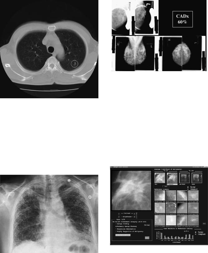
There are several different methods of displaying the CAD output to the radiologist. Figure 2 shows a CT scan that is annotated with a circle indicating an area that the computer deemed suspicious. This is typical for a CADe system. Different symbols are used by different commercial systems. Figure 3 shows a chest radiograph that is annotated with different symbols to indicate different types of disease states. The symbols also have different sizes indicating the severity of the disease. This type of display can be used for both CADe and CADx systems. Figure 4 shows a simple interface that can be used by a CADx system in
286 COMPUTER-ASSISTED DETECTION AND DIAGNOSIS
Figure 2. Typical output of a CADe system. The circle indicates a region that the computer deemed suspicious, in this case for the presence of a lung cancer in a slice from a CT scan of the thoracic.
which the likelihood of malignancy is shown. Figure 5 shows a more advanced interface that can be used by CADx systems. Here the probability that a lesion is malignant is given numerically and in graphically form what this number means in terms of likelihood of being a malignant or benign lesion. In addition, this interface shows lesions similar to the unknown lesion that are selected from a library of lesions with known pathology. This provides a pictorial representation of the computer
Figure 4. An example of a simple interface that could be used by a CADx scheme. Along with the images showing the lesion being analyzed, the display also shows the computer’s estimated likelihood that the lesion is malignant. The images in the top left corner are spot magnification views and the images along the bottom are the standard screening views.
result that to the radiologist may be more intuitive than just a number.
In CADe, lesions or disease states are identified in images. The output of CADe schemes is typically locations of areas that the computer considers suspicious. These areas can then be annotated on the digital image. For CADe, the computer can detect actual lesions (true-positive detection), miss an actual lesion (false-negative detection), or detect something that is not an actual lesion (falsepositive detection). The objective of the computer algorithm is to find all the actual lesions while minimizing the
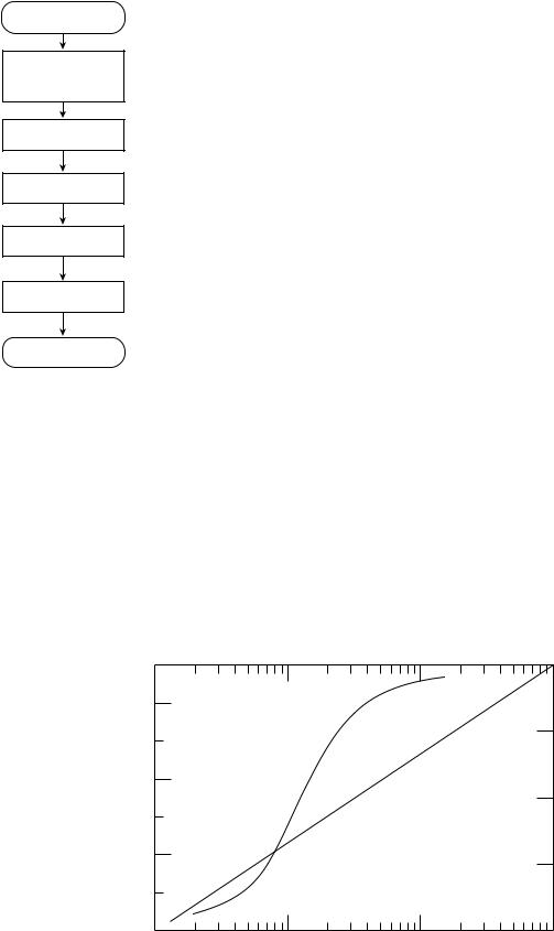
Figure 3. This chest radiograph is annotated with symbols indicating the presence of different appearances or patterns associated with interstitial chest disease. Crosses indicate a normal pattern; squares indicate a reticular pattern, circles represent a nodular pattern; and hexagons are honeycomb or reticulonodular patterns.
Figure 5. An example of an advanced CADx display that shows in addition to the likelihood of malignancy, a graphical representation and a selection of lesions similar to the lesion being examined recalled from a reference library containing lesions with known pathology. The red frame around a lesion indicates a malignant lesion and a green frame indicates a benign lesion.
number of false-positive detections. In practice, there exists a tradeoff between having high sensitivity (high true-positive detections) and the number of false detections per image. This tradeoff is important because the clinical utility of CADe depends on how well the algorithm works. In particular, if the false-positive rate is high (the exact definition of high is unknown) then the radiologist will spend unneeded time examining computer false-detections. Further, there is a possibility that a computer false detection could cause the radiologist to make an incorrect interpretation, if the radiologist should incorrectly agree with the computer. If the sensitivity of the CADe scheme is not high enough, then the radiologist could lose confidence in the CADe scheme’s ability to detect actual lesions, reducing the potential effectiveness of the CADe scheme.
In CADx, the computer classifies different pathologies or different types of diseases. The most common application is to distinguish between benign and malignant lesions, to assist radiologists in deciding which patients need biopsies. The output of a CADx scheme is the probability that a lesion is malignant. If one sets a threshold probability value above which the lesion is considered malignant, the computer classification can be a true-positive (an actual malignant lesion is classified as malignant), a false-negative (an actual malignant lesion is classified as benign), a false positive (an actual benign lesion is classified as malignant), or a true negative (an actual benign lesion is classified as benign). The goal is to maximize the truepositive rate while minimizing the false-positive rate. Both false positives and false negatives could have serious consequences. A computer false positive could influence the radiologist to recommend a biopsy for a patient who does not need one. A computer false negative could influence the radiologist not to recommend a biopsy for a patient who has cancer.
There are important differences between CADx and CADe. In CADe, the results are presented as annotations on an image, so the radiologist examines image data, which they are trained and accustomed to do. In CADx, the output can be in numerical form, which radiologists are neither trained nor accustomed to using. Therefore, it may be more difficult for radiologists to use CADx effectively compared to using CADe. In addition, the consequences of inducing an error by the radiologist is much more severe in CADx than CADe. In most situations, the next step in a positive detection (CADe case) is more imaging, whereas in the CADx case, the next step is usually a biopsy or some other invasive procedure.
Why Is Computer-Aided Diagnosis Needed?
The goal of CAD is threefold: (1) to improve the accuracy of radiologists; (2) to make a radiologist more consistent (reduce intrareader variability) and to reduce discrepancies between radiologists (reduce interreader variability); and (3) to improve the efficiency of radiologists.
Since the interpretation of a radiograph is subjective, even highly trained radiologists make mistakes. The radiographic indication for the presence of a disease is often very subtle because variation in appearance of normal tissue often mimics subtle disease conditions. Another reason a
COMPUTER-ASSISTED DETECTION AND DIAGNOSIS |
287 |
radiologist may miss a lesion is that there is some other feature in the image that attracts their attention first. This is known as satisfaction of search and can occur when, for example, the radiologist’s attention is focused on identifying pneumonia in a chest radiograph so that they do not notice a small lung cancer. Furthermore, in many instances the prevalence of disease in a population of patients is low. For example, in screening mammography only 0.4% of women who have a mammogram actually have cancer. It can be difficult to be ever vigilant to find the often-subtle indications of malignancy on the mammogram. Consequently, the missed cancer rate in screening mammography is between 5% and 35% (13–15) and, in chest radiography, the missed rate for lung cancer is30% (16).
Radiologists often have to decide whether an abnormal area is an indication of malignancy or of some benign process, or they may have to differentiate between different types of diseases that could give rise to the abnormality. This differentiation is often difficult because the radiographic indications between different disease types are not distinct. In diagnosing breast cancer, radiologists will recommend between 2 and 10 breast biopsies of benign lesions or normal tissue for every 1 cancer biopsied (17,18). The 50–90% of women who do not have breast cancer, but undergo a breast biopsy, suffer physical and mental trauma, and valuable medical resources were used unnecessarily. It is estimated that there is a 18.6% chance of receiving a biopsy for a benign condition after 10 years of screening for women in the United States (19). In general, the European false-positive rates are lower than in the United States (20). This is due in part to having a national programs and screening policies in Europe (21) and the higher likelihood of having malpractice lawsuit for a false-negative diagnosis in the United States.
Variability in performance of radiologists will reduce the effectiveness of the radiographic exam and, further, it will undermine the confidence that the public and medical community has in the technology. Again, because of differences in ability and differences in opinions, there exists variability between radiologists. In mammography, the variability between radiologists is well documented and can be very large (up to 40% variation in sensitivity in one national study) (22). Even a given radiologist is not always internally consistent. That is, the same radiologist may give a different interpretation when reading the same case a second time (23).
As the cost of the health care system increases, there is growing pressure to improve the efficiency of the system. In radiology, technology improvements have been introduced to improve workflow. Two examples are digital imaging systems, which can acquire images faster than conventional film systems and picture archive and retrieval systems (PACS), which can streamline the process of storing and recalling images. These and other technology improvements have increased the radiologists’ workload. While not yet proven, it is hoped that CAD will allow the radiologist to read faster without reducing their accuracy. This will probably occur when the CAD schemes reach a certain level of accuracy (the exact level is unknown), so that the radiologist is not spending too much
288 COMPUTER-ASSISTED DETECTION AND DIAGNOSIS
Digital image
Pre-processing (e.g., filtering, organ
segmentation)
Signal identification
Signal segmentation
Feature extraction
Feature analysis
CAD output
Figure 6. A flowchart of a generic CAD scheme. Most CADx and CADe schemes follow this template, although there are widely varying techniques for implementing each step.
time examining– considering computer falsepositives. The CAD may also increase the radiologists’ confidence in their interpretation, which should lead to faster reading times.
COMPUTER-AIDED DIAGNOSIS ALGORITHMS
There are probably thousands of publications on CAD, with hundreds of different techniques being developed. It is not practical to describe them all. There is, however, commonality between most approaches. Most techniques,
whether they are for CADe or for CADx, can be described generically, as outlined in Fig. 6, as consisting of five steps: preprocessing, identification of candidate lesions (signals), segmentation of signals, feature extraction, and classification to distinguish actual lesions from false lesions or to differentiate between different types of pathologies or diseases (e.g., benign and malignant).
Radiographs can either be acquired using digital technology or screen-film systems. In digital systems, the image is acquired as a 2D array of numbers. Each element of the array is a pixel and corresponds to the amount of X-ray energy absorbed in the detector at that pixel location. This in turn is related to the number of X rays transmitted through the patient. Thus, a radiograph is a map of the X-ray attenuation properties of the patient. Different tissues in the body and different tissue pathologies have different attenuation properties, although the differences can be small. In a screen-film system, the image is recorded on X-ray film. The screen converts the X rays into visible light and the light is recorded by the film. For CAD purposes, this film must be digitized so that the image can be analyzed. A film digitizer basically shines light through the film and measures the amount of light transmitted. The resulting image is again a 2D array of numbers related to the X-ray attenuation properties of the patient.
One complicating property of screen-film systems is that they respond nonlinearly to X-ray exposure: digital systems respond linearly. Figure 7 shows the characteristic curve for screen-film system and a digital system. The contrast of objects in the image is proportional to the slope of the characteristic curve. For a screen-film system, at high and low exposures, slope approaches zero. Thus, for screen-film systems the contrast in the image is reduce in bright and dark areas of the image.
In this article, one approach to accomplishing these steps will be illustrated. In general, the techniques described are relatively simplistic, but are used to illustrate the concepts involved. More advanced and effective techniques are described in the literature; in particular,
Figure 7. Comparison of a linear and a nonlinear detector. In a nonlinear detector (e.g., a screen-film system, the response of the system is X-ray exposure dependent. That is, the amount of darkening on the film (called filmoptical density) depends on the X-ray exposure to the detector. At low exposures and high exposures, the image contrast (difference in film optical density)islowerthanatoptimalexposures. For a linear detector (e.g., most digital X-ray detectors), the response of the system is linearly dependent on the X-ray exposure to the detector. As a result, the contrast is independent of X-ray exposure.
Optical density
3
2
1
0
1
Screen-film
system
Digital system
10 |
100 |
Relative exposure
4000
3000
2000
1000
0
1000
Pixel value
review articles (24–29), and conference proceedings, such as the Proceedings of the SPIE Medical Imaging Conference, International Workshop on Digital Mammography (30–35), and the Proceedings of Computer Applications in Radiology and Surgery (CARS).
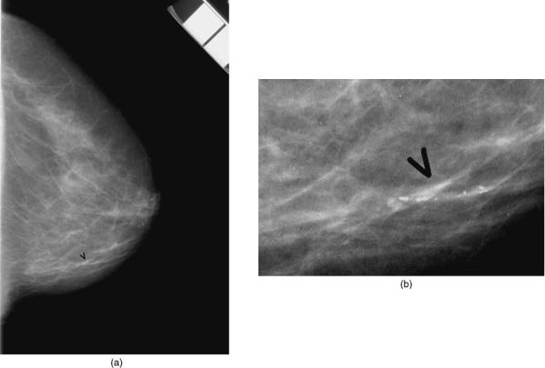
Using a mammogram, the steps outlined in Fig. 6 are illustrated in Figs. 8–14 using a somewhat simple procedure. Figure 8a shows the mammogram with an arrow indicating the location of a cluster of calcifications. An enlargement of the cluster is shown in Fig. 8b. In a radiograph, dark regions correspond to areas where there are more X-rays incident on the image and these are assigned high pixel values; and bright areas correspond to areas with fewer X-rays incident and they are assigned low pixel values. Within the breast area of the image, dark areas correspond to predominately fatty areas of the breast and bright areas correspond to fibroglandular tissues (those involved in milk production and the physical support of the breast to the chest wall). In the following sections, this image will be used to illustrate some of the basic concepts in developing CAD schemes.
Most of the initial CAD research was applied to 2D images, in which the 3D body part is projected into a 2D plane to produce an image. While being relatively simple, fast, and inexpensive, 2-D imaging methods are limited by the superposition of tissue. Lesions can be obscured by overlapping tissues or the appearance of a lesion can be created where no lesion actually exists. Three-dimensional
COMPUTER-ASSISTED DETECTION AND DIAGNOSIS |
289 |
imaging [ultrasound, CT, magnetic resonance imaging (MRI), positron emission tomography (PET), and single- photon-emission competed tomography (SPECT)] produces a 3D image of the body, which is often viewed as a series of thin slices through the body. These images are more costly to produce and take significantly longer to complete the exam, however, they can produce vastly superior images. These image sets also take longer to read. In some cases, the radiologist needs to review up to 400 image slices for each exam. With such large datasets, it is believed that CAD may be beneficial for radiologists.
In developing these techniques, researchers use information that a radiologist uses, information that cannot be visualized by radiologists, and information based on the radiographic properties of the tissue and of the imaging system.
Preprocessing
The first step in a CAD scheme is usually preprocessing. Preprocessing is employed mainly for three reasons: (1) To reduce the effects of the normal anatomy, which acts as a camouflaging background to lesions of interest: (2) To increase the visibility of lesions or a particular feature of a lesion: (3) To isolate a specific region within the whole image to analyze (e.g., the lung field from a chest radiograph). This reduces the size of the image that needs to be analyzed reducing computation time, reducing the chances
Figure 8. (a) A portion of a digitized mammogram. The arrow indicates the location of a cluster of calcifications. (b) An enlargement of the area containing calcifications.

290 COMPUTER-ASSISTED DETECTION AND DIAGNOSIS
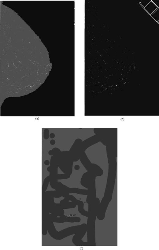
Figure 9. (a) A gray-level threshold was applied to the image shown in Fig. 8 in order to determine the breast boundary. Above the threshold value the image is made white and below the boundary the image is made black. The interface between the two areas is the skinline or breast boundary. (b) The determined breast boundary superimposed on the original image.
of a false detection, and reducing the complexity of the analysis, since only the area of interest is analyzed and extraneous image data are eliminated.
In our example CAD scheme, two procedures are performed. The first is to identify the border of the breast and the second is to process the image to reduce the background structure of the breast so as to highlight small bright areas that could be calcifications. The border of the breast was determined, so as to include only breast area in subsequent analysis. Outside of the breast, the image is black, corresponding to a large number of X rays incident on the film. Within the breast, X rays are absorbed or scattered so that the number of X rays incident on film is decreased and the image appears brighter. In this simple example, the breast outline is determined by thresholding the image so that below a threshold pixel value, all the pixel values are black and equal to above the threshold all pixels are white (Fig. 9a). The border between the black and white pixels is chosen as the border of the breast. The result is shown in Fig. 9b. This method produces a suboptimal result. At the top left corner of the image, there is an area included that does not contain breast tissue that was considered to be part of the breast. When the film was digitized, where there was a sharp transition from bright to dark, the response of the digitizer was slow, so that some of the bright area ‘‘bleeds’’ into the dark area.
In our example, the image is next processed by using a technique called the difference of Gaussians (DoG). In this technique, the image, which is typically 18 24 cm, is filtered twice by Gaussian filters, one with a small width (fwhm value, of 0.155 mm) and the other with a wider width (fwhm of 0.233 mm) (36). The first filter keeps small bright signals in the image (Fig. 10a) and the second eliminates the small bright signals (Fig. 10b). The two images are subtracted producing an image where large structures are eliminated and small signals are retained (Fig. 10c). Another useful outcome of this difference method is that the background of the subtracted image is more uniform compared to the original mammogram. This is important for the next step where potential calcifications are identified using a gray-level threshold method.
Note that for images that are recorded not on film but are acquired in digital format (i.e., a digital mammogram) now undergo preprocessing before the radiologist views the image (37). The goal is to improve the visibility of abnormalities for the human viewer. The techniques used in this type of preprocessing can be similar to those used in preprocessing for CAD purposes. The main difference is that a CAD preprocessed image would be considered overprocessed to the radiologist because they are designed to highlight only one type of lesion, whereas a radiologist needs to look for several to many different types of abnormalities in the image.

COMPUTER-ASSISTED DETECTION AND DIAGNOSIS |
291 |
Figure 10. An example of a preprocessing method using the difference of Gaussian technique. (a) The image shown in Fig. 8 is filtered by a Gaussian filter that has a full width at half-maximum (fwhm) value of 0.155 mm. This filter enhances small objects on the order of 0.5 mm in diameter. (b) The image shown in Fig. 8 is filtered by a Gaussian filter that has a fwhm value of 0.233 mm. This filter degrades small objects on the order of 0.5 mm in diameter. (c) The image in Fig. 10b is subtracted from Fig. 10a producing an image with enhancement of small objects on the order of 0.5 mm in diameter and a reduction in the normal background structure of the breast.
292 COMPUTER-ASSISTED DETECTION AND DIAGNOSIS
Figure 11. An illustration of signal identification using gray-level thresholding. Using the preprocessed image (Fig. 10c), a gray-level threshold is chosen so as to keep only a fraction of the brightest pixels. Three different threshold levels are shown in a–c. If the threshold value is too low as in part a, too many false signals (noncalcifications) will be kept. If the threshold is too high, as in part c, some of the actual calcifications are lost, even though most of the false signals are eliminated.
Number of occurences
COMPUTER-ASSISTED DETECTION AND DIAGNOSIS |
293 |
3.0x10⁻²
2.5 |
|
|
|
|
|
|
|
|
|
|
|
|
|
|
|
|
|
|
|
|
|
|
|
|
|
|
|
|
|
|
|
|
|
|
|
|
|
|
|
|
|
|
|
|
|
|
|
|
|
|
|
|
|
|
|
|
|
|
|
|
|
|
|
|
|
|
|
|
|
|
|
|
|
|
|
|
|
|
|
|
|
|
|
|
|
|
|
|
|
|
|
|
|
|
|
|
|
|
|
|
|
|
|
|
|
|
|
|
|
|
|
|
|
|
|
|
|
|
|
|
|
|
|
|
|
|
|
|
|
|
|
|
|
|
|
|
|
|
|
|
|
|
|
2.0 |
|
|
|
|
|
|
|
|
|
|
|
|
|
|
|
|
|
|
|
|
|
|
|
|
|
|
|
|
|
|
|
|
|
|
|
|
|
|
|
|
|
|
|
|
|
|
|
|
|
|
|
|
|
|
|
|
|
|
|
|
|
|
|
|
|
|
|
|
|
|
|
1.5 |
|
|
|
|
|
|
|
|
|
|
|
|
|
|
|
|
|
|
|
|
|
|
|
|
|
|
|
|
|
|
|
|
|
|
|
|
|
|
|
|
|
|
|
|
|
|
|
|
|
|
|
|
|
|
|
|
|
|
|
|
|
|
|
|
|
|
|
|
|
|
|
|
|
|
|
|
|
|
|
|
|
|
|
|
|
|
|
|
|
|
|
|
|
|
|
|
|
|
|
|
|
|
|
|
|
|
|
|
|
|
|
|
|
|
|
|
|
|
|
|
|
|
|
|
|
|
|
|
|
|
|
|
|
|
|
|
|
|
|
|
|
|
|
1.0 |
|
|
|
|
|
|
|
|
|
|
|
|
|
|
|
|
|
|
|
|
|
|
|
|
|
|
|
|
|
|
|
|
|
|
|
|
|
|
|
|
|
|
|
|
|
|
|
|
|
|
|
|
|
|
|
|
|
|
|
|
|
|
|
|
|
|
|
|
|
|
|
|
|
|
|
|
|
|
|
|
|
|
|
|
|
|
|
|
|
|
|
|
|
|
|
|
|
|
|
|
|
|
|
|
|
|
|
|
|
|
|
|
|
|
|
|
|
|
|
|
|
|
|
|
|
|
|
|
|
|
|
|
|
|
|
|
|
|
|
|
|
|
|
|
|
|
|
|
|
|
|
|
|
|
|
|
|
|
|
|
|
|
|
|
|
|
|
|
|
|
|
|
|
|
|
|
|
|
|
|
|
|
|
|
|
|
|
|
|
|
|
|
|
|
|
|
|
|
|
|
|
|
|
|
|
|
|
|
|
|
|
|
|
|
|
0.5 |
|
|
|
|
|
|
|
|
|
|
|
|
|
|
|
|
|
|
|
|
|
|
|
|
|
|
|
|
|
|
|
|
|
|
|
|
|
|
|
|
|
|
|
|
|
|
|
|
|
|
|
|
|
|
|
|
|
|
|
|
|
|
|
|
|
|
|
|
|
|
Figure 12. A histogram of pixel values from a |
0.0 |
|
|
|
|
|
|
|
|
|
|
|
|
|
|
|
|
|
|
|
|
|
|
|
|
|
|
|
|
|
|
|
|
|
|
|
|
|
|
|
|
|
|
|
|
|
|
|
|
|
|
|
|
|
|
|
|
|
|
|
|
|
|
|
|
|
|
|
|
|
|
|
500 |
550 |
600 |
|
650 |
700 |
|
750 |
800 hypothetical lesion. From a histogram like this |
|||||||||||||||||||||||||||||||||||||||||||||||||||||||||||||||
|
|
|
|
|
|
|
|
|
|
|
|
|
|
|
|
|
|
|
|
|
|
|
|
|
|
|
|
|
|
|
|
|
|
|
|
|
|
|
Pixel value |
|
|
|
|
|
|
|
|
|
|
|
|
|
|
|
|
|
|
|
|
|
one, features can be determined (e.g., mean |
||||||||||
|
|
|
|
|
|
|
|
|
|
|
|
|
|
|
|
|
|
|
|
|
|
|
|
|
|
|
|
|
|
|
|
|
|
|
|
|
|
|
|
|
|
|
|
|
|
|
|
|
|
|
|
|
|
|
|
|
|
|
|
pixel value and kurtosis). See text for details. |
|||||||||||
If the system does not respond linearly to X-ray exposure, then, the background level will affect the image contrast of lesions (see Fig. 7). In bright or dark areas of the image, the contrast is reduced compared to regions that are optimally exposed. This reduces the effectiveness of pixel-value-based and contrast-dependent techniques.
A limitation of these types of filtering is that lesions can often range in size. For example, lung nodules can as small as 0.5 cm or less and 5 cm or larger. A fixed-sized filter cannot be optimal for the full range of sizes possible. To accommodate a large size range, many researchers have developed multiscaled approaches. Wavelets are one class of multiscale filters. Multiple numbers of bandpass filters can be chosen based on which daughter wavelet decomposition are used in reconstructing the image. The principle of applying wavelets to medical images is discussed by Merkle et al. (38). In mammography, a weighted
sum of the different levels in the wavelet domain is performed to enhance calcifications (39). Different approaches differ in their choice of wavelets and the selection of which levels to use in the reconstruction. A list of different wavelets used for processing microcalcifications on mammograms is given in Table 1.
Identification of Lesions
Once the image has been preprocessed, candidate lesions or signals need to be identified. The goal in CADe is to maximize the number of actual lesions identified even if a large number of false signals are detected. The false detections are reduced in the feature analysis step.
Signal identification is sometimes accomplished simultaneously with lesion segmentation (see next section). However, there are circumstances in which it is not. The
Relative contrast
0.20
0.15
0.10 |
|
|
|
|
|
|
|
|
|
|
|
|
|
|
|
|
|
|
|
|
|
|
|
|
|
|
|
|
|
|
|
|
|
|
|
|
|
|
|
|
|
|
|
|
|
|
|
|
|
|
|
|
|
|
|
|
|
|
|
|
|
|
|
|
|
|
|
|
|
|
|
|
|
|
|
|
|
|
|
|
|
|
|
|
|
Figure 13. An example of feature analysis |
|
|
|
|
|
|
|
|
|
|
|
|
|
|
|
|
|
|
|
|
|
|
|
|
|
|
|
|
|
|
|
|
|
|
|
|
|
|
|
|
|
|
|
|
|
|
|
|
|
|
|
|
|
|
|
|
|
|
|
|
|
|
|
|
|
|
|
|
|
|
|
|
|
|
|
|
|
|
|
|
|
|
|
|
|
||
|
|
|
|
|
|
|
|
|
|
|
|
|
|
|
|
|
|
|
|
|
|
|
|
|
|
|
|
|
|
|
|
|
|
|
|
|
|
|
|
|
|
|
|
|
|
|
|
|
|
|
|
|
|
|
|
|
|
|
|
|
|
|
|
|
|
|
|
|
|
|
|
|
|
|
|
|
|
|
|
|
|
|
|
|
|
|
|
|
|
|
|
|
|
|
|
|
|
|
|
|
|
|
|
|
|
|
|
|
|
|
|
|
|
|
|
|
|
|
|
|
|
|
|
|
|
|
|
|
|
|
|
|
|
|
|
|
|
|
|
|
|
|
|
|
|
|
|
|
|
|
|
|
|
|
|
|
|
|
|
|
|
|
|
|
|
|
|
|
|
|
|
|
|
|
|
|
|
|
|
|
|
|
|
|
|
|
|
|
|
|
|
|
|
|
|
|
|
|
|
|
|
|
|
|
|
|
|
|
|
|
|
|
|
|
|
|
|
|
|
|
|
|
|
|
|
|
|
|
|
|
|
|
|
|
|
|
|
|
|
|
|
|
|
|
|
|
|
|
|
|
|
|
|
|
|
|
|
|
|
|
|
|
|
|
|
|
|
|
|
|
|
|
|
|
|
|
|
|
|
|
|
|
|
|
|
|
|
|
|
|
|
|
|
|
|
|
|
|
|
|
|
|
|
|
|
|
|
|
|
|
|
|
|
|
|
|
|
|
|
|
|
|
|
|
|
|
|
|
|
|
|
|
|
|
|
|
|
|
|
|
|
|
|
|
|
|
|
0.05 |
|
|
|
|
|
|
|
|
|
|
|
|
|
|
|
|
|
|
|
|
|
|
|
|
|
|
|
|
|
|
|
|
|
|
|
|
|
|
|
|
|
|
|
|
|
|
|
|
|
|
|
|
|
|
|
|
|
|
|
|
|
|
|
|
|
|
|
|
|
|
|
|
|
|
|
|
|
|
|
|
|
|
|
|
|
in which two features, contrast and size, are |
|
|
|
|
|
|
|
|
|
|
|
|
|
|
|
|
|
|
|
|
|
|
|
|
|
|
|
|
|
|
|
|
|
|
|
|
|
|
|
|
|
|
|
|
|
|
|
|
|
|
|
|
|
|
|
|
|
|
|
|
|
|
|
|
|
|
|
|
True signals |
|
|
|
|
used to differentiate actual calcifications |
|||||||||||||
|
|
|
|
|
|
|
|
|
|
|
|
|
|
|
|
|
|
|
|
|
|
|
|
|
|
|
|
|
|
|
|
|
|
|
|
|
|
|
|
|
|
|
|
|
|
|
|
|
|
|
|
|
|
|
|
|
|
|
|
|
|
|
|
|
|
|
|
|
False signals |
|
|
|
|
from computer-detected false detections. A |
||||||||||||
|
|
|
|
|
|
|
|
|
|
|
|
|
|
|
|
|
|
|
|
|
|
|
|
|
|
|
|
|
|
|
|
|
|
|
|
|
|
|
|
|
|
|
|
|
|
|
|
|
|
|
|
|
|
|
|
|
|
|
|
|
|
|
|
|
|
|
|
|
|
wave0 |
|
|
|
|
|
|
|
|
|
|
|
|
|
threshold can applied to reduce the number |
||
0.00 |
|
|
|
|
|
|
|
|
|
|
|
|
|
|
|
|
|
|
|
|
|
|
|
|
|
|
|
|
|
|
|
|
|
|
|
|
|
|
|
|
|
|
|
|
|
|
|
|
|
|
|
|
|
|
|
|
|
|
|
|
|
|
|
|
|
|
|
|
|
|
|
|
|
|
|
|
|
|
|
|
|
|
of false detections, without eliminating |
|||
|
|
|
|
|
|
|
|
|
|
|
|
|
|
|
|
|
|
|
|
|
|
|
|
|
|
|
|
|
|
|
|
|
|
|
|
|
|
|
|
|
|
|
|
|
|
|
|
|
|
|
|
|
|
|
|
|
|
|
|
|
|
|
|
|
|
|
|
|
|
|
|
|
|
|
|
|
|
|
|
|
|
|||||
|
|
|
|
|
|
|
|
|
|
|
|
|
|
|
|
|
|
|
|
|
|
|
|
|
|
|
|
|
|
|
|
|
|
|
|
|
|
|
|
|
|
|
|
|
|
|
|
|
|
|
|
|
|
|
|
|
|
|
|
|
|
|
|
|
|
|
|
|
|
|
|
|
|
|
|
|
|
|
|
|
|
|
|
|
many actual calcifications. In this example, |
|
|
|
|
|
|
|
|
|
|
|
|
|
|
|
|
|
|
|
|
|
|
|
|
|
|
|
|
|
|
|
|
|
|
|
|
|
|
|
|
|
|
|
|
|
|
|
|
|
|
|
|
|
|
|
|
|
|
|
|
|
|
|
|
|
|
|
|
|
|
|
|
|
|
|
|
|
|
|
|
|
|
|
|
|
|
||
0.0 |
0.2 |
|
|
|
|
|
|
0.4 |
|
0.6 |
|
|
|
|
|
|
0.8 |
|
|
|
1.0 |
1.2 |
|
1.4 the broken straight line shows the threshold |
||||||||||||||||||||||||||||||||||||||||||||||||||||||||||||||
|
|
|
|
|
|
|
|
|
|
|
|
|
|
|
|
|
|
|
|
|
|
|
|
|
|
|
|
|
|
Effective size (mm) |
|
|
|
|
|
|
|
|
|
|
|
|
|
|
|
|
|
|
|
|
|
|
values. |
|||||||||||||||||||||||||||||||||

294 COMPUTER-ASSISTED DETECTION AND DIAGNOSIS
Figure 14. An example of the output of a simple CADe method illustrated in Figs. 8–13. This simple method detected the actual cluster of calcifications, but also two false clusters. More sophisticated methods can have much better performance over a wide variety of cases.
most obvious case is when a human indicates the location of signals. When functioning clinically a CADx scheme needs to know the location of the lesion that needs to be classified. This can be done using a CADe scheme. However, the CADe scheme may not detect a lesion that the radiologist is scrutinizing because either the CADe scheme may have failed to detect the lesion or the area that the radiologist is examining does not contain a real lesion. In either case, the radiologist would have to mark the location of the lesion in order for the CADx scheme to analyze it. When this occurs, the process is no longer automated.
Table 1. List of Different Mother Wavelets Used for Processing Mammograms Containing Microcalcifications
Lead Investigator |
Reference |
Wavelet |
|
|
|
Brown |
40 |
Undecimated spline |
Chen |
41 |
Morlet |
Chitre |
42 |
Daubechies’ 6- and |
|
|
20coefficient |
Kallergi |
43 |
12-coefficient Symmlet |
Laine |
44 |
Dyadic |
Lo |
45 |
Daubechies 8-tap |
Strickland |
46 |
Biorthogonal B-spline |
Wang |
47 |
Daubechies’ 4- and |
|
|
20coefficient |
Yoshida |
48 |
8-tap least |
asymmetric Daubechies
In X-ray imaging, the presence of a disease state is usually detected because the lesion is either more attenuating or less attenuating than the surrounding tissue. That is the lesion that will appear as a bright or a dark spot in the image. This makes gray-level thresholding a potentially useful method for segmentation. In Fig. 11, our example image has undergone gray-level thresholding using different thresholds. As the threshold is increased the total number of detections decrease. If the threshold is too high, some actual calcifications are lost. The signals that are detected that do not correspond to actual calcifications are caused by primarily image noise (due to the statistical fluctuations in the number of X rays incident on the patient per unit area) and normal breast tissue. Unfortunately, radiographs are a 2D projection of a 3D object, so that summation of overlapping tissues can produce areas in the image that mimic actual lesions. While gray-level thresholding can be effective on a given image, over a large number of images this simple thresholding method is not optimal. Calcifications can appear differently in different images, due in part to differences in the X-ray exposure used to make the image. Therefore, a single threshold applied to a cross-section of images will not be effective.
One method to improve the gray-level thresholding method is to make it adaptive. For example, one can use the statistics of a small region (e.g., 5 mm2) centered on the calcification to select the appropriate threshold (2). A threshold can be set to the mean pixel value within the region plus a multiple (typically 3.0–4.0) of the standard deviation within the region. In this way, differences in X-ray exposure and differences in image noise can be accounted for.
Lesion Segmentation
Once the location of a lesion has been determined, the exact border of the lesion needs to be determined. This is necessary to extract features of the lesion. Again, gray-level threshold can be employed. One simple method is to find the highest pixel value near the identified pixel (e.g., in a 0.3 0.3 mm region) and then to find the mean pixel value in a local area surrounding the signal (e.g., in a 1 1 cm region). A threshold can be taken to be the mean pixel value, plus 50% of the difference between the maximum pixel value and the mean pixel value. Finally, all pixels above the threshold that are connected to the pixel with the maximum value are considered to be part of the calcification. Starting from a seed point, in this case the pixel with the highest value, a region is grown that contains all connected pixels that are above threshold. Connected pixels can be defined as the pixel above, below, to the right, and to the left of a given pixel, so-called four-point or eightpoint connectivity, the same four pixels plus the four corner pixels.
This region growing method can be improved by first correcting the appearance of the calcification in the image for the degradation caused by the imaging system. The imaging will blur the image and further, the imaging system can response nonlinearly to X-ray exposure. Jiang et al. (49), and Veldkamp and Karssemeijer (50) indepen-
dently developed a segmentation technique based on background-trend correction and signal dependent thresholding. In these two approaches, corrections for the nonlinear response and the blurring of the calcification by the screen-film system and film digitizer are performed. At low and high X-ray exposures to the screen, the contrast, which is proportional to the slope of the characteristic curve, is reduced (see Fig. 7). That is, the inherent contrast of the calcifications is reduced when recorded by the screen-film system. Therefore, the image or radiographic contrast will depend on the background intensity. If a correction is not made for this nonlinearity, then it becomes extremely difficult to segment accurately calcifications in dense and fatty regions of the image simultaneously with calcifications in other regions of the breast. Similarly, the smaller the calcification, the more that its contrast is reduced due to blurring. This can be corrected based on the modulation transfer function of the screen-film system (51).
The above segmentation method will work well as long as there is sufficient separation between the calcifications. If two or more calcifications are too close, then they may be segmented as one large calcification. In such situations, more sophisticated methods are more effective. Besides the pixel value, thresholding can be applied based on other features of the image, such as the texture and gradients. These more advanced techniques are also important in applications where the border of the lesions is not welldefined visually in the image.
Feature Extraction
To reduce the number of false detections (i.e., to differentiate true lesions from false detections) or to classify a lesion (e.g., benign versus malignant) features are extracted and subsequently used by a classifier. The strategy in CADe is to segment as many actual lesions as possible. This will include a large number of false detections.
There are probably thousands of features that can be used and these are dependent on the imaging task. Further, the optimum set of features is not known for any imaging task. Therefore, a large number of different features are being used by different investigators. The
COMPUTER-ASSISTED DETECTION AND DIAGNOSIS |
295 |
features are based on those that a radiologist would use and those that a radiologist would not use. As an example, a radiologist uses the brightness of the lesion to determine whether a lesion is present in the image. This can be determined conceptually by plotting a histogram of pixel values (see Fig. 12). The brightness is related to the mean pixel value, M, and is given by
|
1 |
N |
|
M ¼ |
|
Xi 1 f ðiÞ pðiÞ |
ð1Þ |
N |
|||
|
|
¼ |
|
where f is the frequency of occurrence of pixel value p(i), N is the total number of pixels in the region being analyzed, and i is the index in the histogram, f(i). An example of a feature not used by a radiologist is kurtosis, K, which is defined as
|
1 |
N |
|
|
|
|
4 |
|
|
|
|
|||
|
iP¼1ð f ðiÞ MÞ |
pðiÞ |
|
|
||||||||||
|
|
|
N |
|
|
|
||||||||
K ¼ |
|
|
|
|
|
|
|
|
|
|
|
|
|
ð2Þ |
1 |
|
N |
|
|
|
2 |
|
# |
2 |
|||||
|
iP¼1ð |
ð Þ |
M |
Þ |
ð Þ |
|
|
|||||||
|
|
|
|
|
|
|
|
|||||||
|
"N |
f i |
|
|
|
p i |
|
|
||||||
The kurtosis describes the flatness of the histogram. Histograms that are very peaked have high kurtosis. Kurtosis can also be thought of as comparing the histogram to a Gaussian distribution. A value of 3.0 indicates that the histogram has a Gaussian distribution.
A large, but incomplete, list of features used by different investigators for the detection of calcifications in mammograms is given in Table 2. The features used for other applications of CADe and CADx will differ than the ones in Table 2, but the categories will be the same: pixel intensity-based, morphology-based, texture-based, and others. For example, for 3D images, such a CT scan of the thorax, instead of a circularity feature, the sphericity of a lesion would be calculated. The drawback of having a large number of features to choose from is that the selection of the optimum set of features is difficult to do, unless a very large number of images are available for feature selection (69). These images are in addition to the images needed for training and the images needed for testing the technique.
Table 2. List of Different Features Used for Distinguishing Actual Calcifications from False Detections
Pixel-Value Based |
Morphology Based |
Derivative Based |
Other |
|
|
|
|
Contrast (52–57) |
Area (52,54,56,58,59) |
Mean edge gradient |
Number of signals per cluster |
|
|
(45,54,55,57,60–64) |
(52,59,65) |
Average pixel value (53,66) |
Area/maximum linear |
Standard deviation of |
Density of signals in cluster |
|
dimension (61) |
gradient (62) |
(52,58,59) |
Maximum value (45,67) |
Average radius (67) |
Gradient direction (64) |
Distance to nearest neighbor (65) |
Moments of gray-level |
Maximum dimension |
Second derivative (55) |
Distance to skin line (65) |
histogram (68) |
(62) |
|
|
Mean background value (45) |
Aspect ratio (65) |
|
Mean distance between signals (59) |
Standard deviation in |
Linearity (63) |
|
First moment of power spectrum (6) |
background (45,57,58) |
|
|
|
Circularity (54,59,67) Compactness (61,53,55) Sphericity (contrast is the
third dimension) (67) Convexity (68)
Effective thickness (49) Peak contrast/area (67) Mean distance from center
of mass (42)
296 COMPUTER-ASSISTED DETECTION AND DIAGNOSIS
Most of the features listed in Table 2 use standard techniques for determining their value. One feature, effective thickness of the calcification developed by Jiang et al., is calculated using a model of image formation (49). That is, what thickness of calcification will give rise to a given measured contrast in the digital image? To do this, corrections for the blurring of the digitizer and the screen-film system are performed, along with corrections for the characteristic curves of the digitizer and the screen-film system. The assumption is that, in general, calcifications are compact, so their diameter and thickness should be comparable. Film artifact (e.g., dust on the screen), will have a very high thickness value compared to its size, and therefore can be eliminated. Similarly, detections that are thin compared to their area are likely to be false positives due to image noise.
Highnam and Brady take this one step further. For every pixel in the image they estimate the corresponding thickness of nonfatty tissue (essentially fibroglandular tissue) by making the corrections described in the preceding paragraph and in addition corrections for X rays that are scattered within the breast, for the energy and intensity distribution of the X-ray beam, and for other sources (70). This in principal produces an effective image that is independent of how the image was acquired or digitized.
Most features are extracted from either the original image or a processed image that has sought to preserve the shape and contrast of the calcifications in the original image. Zheng et al. used a series of topographical layers (n ¼ 3) as a basis for their feature extraction. The layers generated by applying a 1, 1.5, and 2% threshold using equation 2. This allows for features related to differences between layers (e.g., shape factor in layer 2 and shape factor in layer 3) and changes between layers (e.g., growth factor between layers 1 and 2) to be used.
Classification
Once a set of features has been identified, a classifier is used to reduce the number of false detections, while retaining the majority of actual calcifications that were detected. Several different classifiers are being used: simple thresholds (2,52–54,60–62,71), artificial neural networks (40,72–74), nearest-neighbor methods (54,75,76), fuzzy logic (45,68), linear discriminant analysis (77), quadratic classifier (40), Bayesian classifier (55), genetic algorithms (78), and multiobjective genetic algorithms (79).
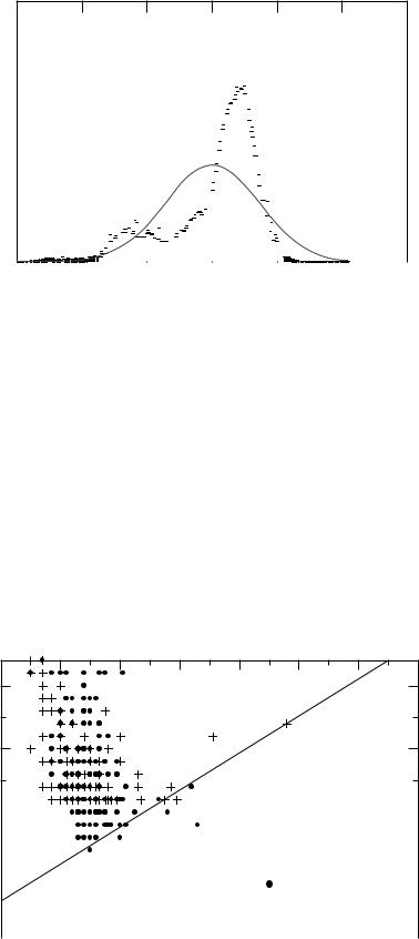
The objective of the classifier is to find the optimal threshold that separates the two classes. Shown in Fig. 13 is an example problem where two features of candidate lesions have been extracted and plotted (2D problem). The classifier determines the boundary between the two classes (normal and abnormal). The optimal boundary is one that maximizes the area under the receiver operating characteristic (ROC) curve (see the section CADx Schemes). There are different types of classifiers: linear, quadratic, parametric, and nonparametric. A linear classifier will produce a boundary that is a straight line in a 2D problem, as shown in Fig. 13. Quadratic classifiers can produce a quadratic line. More complex classifiers (e.g., k nearest
neighbor, artificial neural networks, and support vector machines) can produce very complex boundaries.
Alternatives to Feature Extraction
In lieu of feature extraction, or in addition to feature extraction, several investigators have used the image data as input to a neural network (80–83). The difficulty with this approach is that the networks are usually, quite complex (several thousand connections). Therefore, to properly train the network and to determine the optimum architecture of the network requires a very large database of images.
Another limitation of these and similar approaches is that extremely high performance is needed to avoid having a high false-positive rate. The vast majority of mammograms are normal and the vast majority of the areas of mammograms that are abnormal do not contain calcifications. Mammographically, the average breast is 100 cm2 in area. For a 50 mm pixel, there will be 4 million pixels to be analyzed. If there are 13 calcifications of 500 mm in diameter, then only 0.01% of pixels will belong to a calcification. Therefore, a specificity of 99.9% will give rise to 10 false ROIs per image, which is more than 100 times higher than a radiologist.
Computation Times
The computation times are not often stated by most investigators, perhaps under the belief that this is not an important factor since computers will always get faster. In general, times range from 20 s (84) up to several tens of minutes (inferred from description of other published techniques), depending on the platform and pixel size of the image. For any of the technique to be used clinically, they must be able to process images at a rate that is useful clinically. For real-time analysis (e.g., for diagnostic mammography) there is approximately one patient approximately every 20 min per X-ray machine. This means there is 5 min available per film, including the time to digitize the film. However, many clinics have several mammography units, and some clinics have mobile vans that image up to 200 women off-site. In these situations, computation times of <1 min per film may be necessary or multiple CADe systems would need to be employed. This also assumes that only one detection scheme is run. In mammography, at least one other algorithm, for the detection of masses, will be implemented, cutting the available time for computation in half.
In most centers, screening mammograms are not read to the next day. This allows for processing overnight and computation time becomes less critical, but still important. To analyze 20 cases (80 films) in 15 h (overnight) is 11 min per film for at least two different algorithms. For a higher volume center (40 cases), this gives <3 min for each algorithm.
In other applications, the results of the computer analysis are needed immediately. For example, if a radiologist marks in the image an area that they would like analyzed by the computer (e.g., to determine the likelihood of malignancy of a lesion) then the radiologist, who is busy and under pressure to read the images quickly and accurately, does not want to wait to see the computer results. If the
computer takes more than a few seconds to return a result to the radiologist, then the radiologist may choose not to use the computer because it is reducing down their productivity. Computation time is not a trivial matter.
EVALUATION OF CAD ALGORITHMS
CADx Schemes
The performance of a CADx scheme can be measured in terms of sensitivity (the fraction of actual abnormal cases that are called true) and specificity (the fraction of actual normal cases called normal). This pair of values is easy to compute. However, in general, as the sensitivity increases, the specificity decreases. This can give rise to the problem of comparing two CADx schemes, one with high sensitivity, but low specificity, and the other with lower sensitivity, but higher specificity. This problem is solved by using ROC analysis (85,86).
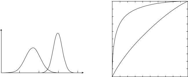
The CADx schemes that involve a differentiation between two categories or classes (e.g., benign and malignant) can be evaluated using ROC analysis. In a two-class classification, objects are separated into one of two classes. This is usually done based on feature vector that characterized the object. Conceptually, the problem reduces to sorting lesions into one of two classes based on the feature vector as illustrated in Fig. 15. In any problem of interest, the population of feature vectors for actual negatives (e.g., benign or computer-detected false-positives) overlaps with the population of feature vectors for actual positives (e.g., malignant or actual lesions). Depending on the selection of a threshold based on a given feature vector value, some actual negatives will be classified as positive and vice versa. Depending on the selected threshold, different pairs of true-positive fraction (the fraction of actual positive cases that are classified as positive) and false-positive fraction
p(C)
Actual positive
Actual negative
C
0.0 |
0.5 |
1.0 |
1.5 |
2.0 |
Figure 15. Conceptual representation of a two-class classification problem. The task is to classify lesions correctly into either actually negative lesions (e.g., benign or computerdetected false positive) or actually positive lesions (e.g., malignant or an actual lesion). The two probability distributions represents the probability of an positive or a negative lesion having a given value of a feature C (contrast). For a small range of contrasts (1.1–1.4), the two distributions overlap and misclassification can occur. To reduce the overlap regions, multiple features, instead of a single feature, are used.
COMPUTER-ASSISTED DETECTION AND DIAGNOSIS |
297 |
(the fraction of actual negative cases that are classified as positive) will be obtained. By selecting all possible thresholds, a set of TPF and FPF pairs will be obtained and they will form an ROC curve, as shown in Fig. 16. In practice, the populations shown in Fig. 15 are not smooth, because only a finite number of cases are used in evaluating a CAD scheme. Therefore, there is some uncertainty as to the true shape of the ROC curve. Fortunately, statistical methods exist to fit a curve to the TPF-FPF pairs (86). The most common summary metric to compare different ROC curves is the area under the curve (AUC). The AUC is the average TPF for all possible FPFs. Since there is uncertainty to the exact shape of the ROC curve, there is uncertainty in the true AUC value. Again, statistical methods have been developed to allow hypothesis testing between curves (86).
The most advanced of the ROC analysis methods can allow generalization of the results to any population of cases that are represented by the testing cases and to a pupulation of readers (87). This is, so-called multiple- reader-multiple-case (MRMC) model is important when analyzing observer studies (see the section Observer Studies).
If the CADx scheme is not a two-class problem, then currently there is no validated method for evaluating the CADx scheme in general (88). One can, however, reduce the problem to a series of two-class problems or make some assumptions to simplify the problem to allow two-class ROC analysis to be used (89–91).
While the AUC is a useful metric, it assumes that all TPF are equally desirable. Often, this is not the case. In diagnostic mammography, where the radiologist must
|
1.0 |
|
|
|
|
|
|
0.8 |
|
|
|
|
|
fraction |
0.6 |
|
|
|
|
|
positive-True |
0.4 |
|
|
|
|
|
|
|
|
|
|
|
|
|
0.2 |
|
|
|
|
|
|
0.0 |
|
|
|
|
|
|
0.0 |
0.2 |
0.4 |
0.6 |
0.8 |
1.0 |
False-positive fraction
Figure 16. A typical ROC curve. The higher curve indicates higher performance than the lower curve. The upper curve represents the performance of radiologists in classifying masses as benign or malignant and it has an area under the curve of 0.91. The lower curve represents the performance of radiologists in classifying calcifications and it has an area under the curve of 0.62.
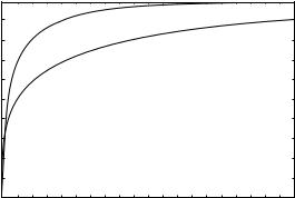
298 COMPUTER-ASSISTED DETECTION AND DIAGNOSIS
decide whether a known breast lesion is benign or malignant, the ‘‘penalty’’ for missing a cancer (classifying a malignant lesion as benign) is considered greater than classifying a benign lesion as malignant. In such circumstances, it may be more appropriate to consider only the region of the ROC curve in the high sensitivity (TPF) region (92,93). Partial AUC can be estimated, for example, considering the area under the curve for TPF >0.80. This would imply that operating at a TPF <0.80 is clinically unacceptable.
Finally, radiologists, when reading clinically, operate at one point on an ROC curve. In fact, two radiologists could have a difference of opinion on a number of cases, but operate on the same ROC curve. If one radiologist is more aggressive than the other, than the aggressive radiologist will have a higher TPF and a higher FPF than a more conservative radiologist and thus would be operating at a point higher up on the curve. Given that AUC is used as a figure of merit, then two radiologists having the same ROC curve have the same performance, although one may detect more disease than the other, because the other radiologist will have a lower false-positive rate (i.e., higher specificity).
CADe Schemes
The CADe schemes are not amenable to ROC analysis because CADe schemes address detection of lesions not the classification of a known lesion as with CADx schemes. That is, lesion classification is often a binary problem (e.g., benign or malignant), and therefore ROC analysis can be used. The CADe schemes involve the identification of the location of a lesion in the image and thus it is not a binary problem. The CADe schemes in general involve a tradeoff between TPF and false-positive rate (the number of false detections per image). Under such situations, free-response operating characteristic (FROC) curves are plotted (94). An example curve is shown in Fig. 17. For the task of detecting a lesion, it is important to identify the location of the lesion correctly. This raises the issue of how to score a CADe detection as correct or a miss (see the section Scoring Criteria).
In an ROC plot, the two axes range between 0 and 1.0, since they represent the true and false positive fractions
|
100 |
|
|
|
|
(%) |
80 |
|
|
|
|
detected |
60 |
|
|
|
|
positives |
|
|
|
|
|
40 |
|
|
|
|
|
|
|
|
|
|
|
True |
20 |
|
|
|
|
|
|
|
|
|
|
|
0 |
|
|
|
|
|
0.0 |
0.5 |
1.0 |
1.5 |
2.0 |
Ave. number of false detections per image
Figure 17. Typical FROC curves. The upper curve represents better performance.
(i.e., they are the ratio of two numbers). In an FROC plot, the y axis ranges from 0 and 1.0, but the x axis can range between 0 and 10 or higher, since there can be multiple detections on one image. That is, the upper limit for the average number of false positives per image is not fixed. Because of this difference between FROC and ROC curves, the statistical methods to analysis ROC data cannot be applied to FROC data. Recently, Chakraborty developed a statistical method for comparing two FROC curves (95), although the method still has some limitations.
In general, CADe schemes are not as accurate as radiologists, because the computer’s false-positive rate is much higher than that of radiologists. Radiologists recall 10% patients who receive a screening mammogram. Since only0.5% of the screened population will have breast cancer, the radiologist has a false-positive rate of 0.0125–0.025 per image (the higher number is assuming that the lesion was seen in both views). The CADe schemes have 10 times higher false-positive rates.
Technical Issues in Evaluation
The measured performance of a CAD scheme is important to compare different CAD schemes. The measured performance of a CAD scheme depends on several factors: (1) the inherent performance of the scheme; (2) the cases used to evaluate the scheme; (3) the scoring criteria used; (4) the quality of the truth data; (5) the method used to develop, train, and evaluate the scheme.
Ideally, one would like factors 2–5 above to be identical in all measurements of performance, but this does not exist at present, since there are no universal standards for these factors. Factors 2–5 are described below.
Database. The measured performance of a CAD scheme depends of the difficulty of cases used to evaluate performance. For a detection scheme, if the cases contain a high fraction of obvious abnormalities, then the measured performance will be high (96). In fact, differences in the cases used for evaluation can easily mask difference in true performance between two different CADe schemes.
The same problem exists for CADx schemes. Here an obvious case would be one that belongs clearly to one of the two classes. Often researchers will use a consecutive series of cases that went to biopsy as an evaluation dataset. These in general, represent difficult cases, especially for the actually benign cases, since at least one radiologist thought the cases was suspicious. However, since different radiologists have different skill levels, a set of consecutive biopsied cases from one institution may be different in difficulty from a set of consecutive biopsied cases from another institution. Currently, there is no method available to compare the difficulty of cases.
Public databases are becoming available (97). There are two websites where images can be downloaded: one for mammograms (http://marathon.csee.usf.edu/Mammography/Database.html) and the other for CT scans of the lungs (http://imaging.cancer.gov/reportsandpublications/ reportsandpresentations/firstdataset). These in principal allow a common set of cases to be used in evaluating CAD schemes. This development is important in allowing
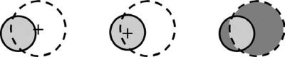
COMPUTER-ASSISTED DETECTION AND DIAGNOSIS |
299 |
comparison of different CAD schemes, but is insufficient in of itself.
Truth. Truth is elusive in CAD research, but vitally important. To optimize and to train a CAD scheme properly, accurate truth information is needed. Truth is needed at several levels. First, the pathology of actual lesions needs to be known (i.e., benign, malignant, or normal tissue). If a biopsy is performed, then it is possible to determine whether a lesion is malignant. However, there is some variability between pathologists, particularly on ‘‘borderline’’ lesions (those on the line between being malignant and premalignant). Further, studies have shown that pathologists, while being highly accurate, make mistakes5% of the times. Researchers usually accept this level of accuracy since it is too time consuming and costly to have the pathology of all biopsies redone.
There are lesions that are potentially malignant, but do not go to biopsy. In these patients, the lesion is followed and either a biopsy is performed in the future when the lesion becomes more suspicious, or the lesion is judged to stable after following the patient with more imaging in subsequent years. However, in a number of instances, the patient moves or changes hospitals and their follow-up is then incomplete. These patients are usually eliminated from CAD research use.
The next level of truth is where is the exact boundary of a lesion. It is not possible to know the answer to this question. Even though the boundary can be well defined by a pathologist, it is not possible to correlate the pathology boundary from the excised tissue to the boundary of the lesion in the image. To optimize (e.g., the segmentation of a lesion), the boundary of the lesion needs to be known exactly, that is, whether a given pixel in the image is part of the lesion or not. The current method to determine ‘‘truth’’ for the boundary of a lesion is to have a radiologist draw the outline of the lesion while viewing the image on a computer screen. Since this is subjective, the variability can be reduced by getting a number of radiologists to outline the lesion.
The last level of truth is whether a lesion is present or not. There are two notable examples of this problem: microcalcifications in a mammogram and lung nodules
in a CT scan. It is possible to know with certainty that a cluster of microcalcifications is present in a mammogram: The tissue containing the cluster that can be seen mammographically is excised and a pathologist can verify that calcifications are present in the tissue. It is not possible, however, to determine the location of every individual calcification in the cluster, even if the pathologist were able to count the number of calcifications in the cluster. When cancer metastasizes to the lungs, it is not possible to determine the exact number of nodules present, because some of the nodules are very subtle and difficult to detect in the images. With metastatic lung cancer, it is not necessary clinically to biopsy every nodule present.
To deal with this uncertainty, a number of radiologists, often called a panel of experts, can mark the location of individual microcalcifications or lung nodules. However, there are a number of problems with using a panel of experts. First, there is wide variability between radiologists, so that a large number of radiologists is needed to form the panel. The minimum number, if not known, is likely >3. Panels can also be biased. Members of the panel can discuss their markings to reduce variability. However, one member of the panel could unduly influence other members of the panel, for example, if one member is a world-renowned expert (98).
Scoring Criteria. For CADx schemes, scoring the computer output is straightforward when ROC analysis is used. The truth for each case is known (either benign or malignant). Then it is a matter of selecting a threshold (applied to the CADx output) for which a lesion is considered malignant. For a given threshold, if the output of the CADx scheme is greater than the threshold value, then the lesion was classified as malignant.
For CADe output, scoring is much more problematic. There are many different criteria used for judging whether the computer found the lesion or whether the detection is a false positive (a computer detection not corresponding to an actual lesion). Most scoring criteria rely on some combination of the location of the center of the computer-detected signal and the actual lesion and the border of the computerdetected signal and the actual lesion. Figure 18 illustrates
Figure 18. An illustration of some different criteria used to score computer detections of actual lesions. The actual lesion is shaded light blue and the computer detection is given by the circle with the dashed line. In the right most figure, the computer is scored as a false detection, since the center of the computer-detected lesion is not within the boundary of the actual lesion. In the center part of the figure, the computer detection is scored as a true positive, since the center of the actual lesion is within the boundary of the computer detection. In this method, there is no penalty when the computer detects a very large lesion, even though the actual lesion may be small. Both of these methods are sensitive to the size of the actual lesion and the computer detected lesion. The method on the right corrects for these effects. In this method the area of the overlap of the computer-detected lesion and the actual lesion (light blue area) is divided by the area of the union of the two lesions (the gray and light blue areas). If this value is greater than a threshold (e.g., 40%), then the computer detection is scored as a true positive.
300 COMPUTER-ASSISTED DETECTION AND DIAGNOSIS
several different scoring methods. There is no consensus on whichis the best method. Inaddition to the objective methods illustrate in the figure, many clinical studies rely on the subjective opinion of a radiologist to determine whether the computer correctly detected the lesion. Given the variability among radiologists, this method has severe limitations.
Methodology. As the field of CAD matures, evaluation methodology is becoming more refined, reducing possible biases that were common in earlier work. It is now known that different sets of images are needed to develop a technique, to train the technique, and to test the technique (69,99,100). However, unlike some other type of image analysis problems, medical images that have verified truth are not easily obtainable. Therefore, while it is desirable to have three independent datasets to develop, train and test, it is usually not possible.
When images are scarce, training and testing can be accomplished through cross-validation or bootstrapping (101–105). These methods divide a single dataset into two subsets: one for training and the other for testing. If the cases are divided such that all images from a given patient are all in one or the other subset, then bias due to commonality of images between testing and training can be eliminated. When dividing the dataset into subsets there are two contrasting goals: maximize the number of training images to properly train the algorithm versus maximizing the number of test images to minimize the variance in the measured performance.
There are three common cross-validation methods used in CAD research:
1.K-fold. The dataset is divided into K subsets of equal size. One of the K subsets is reserved for testing while the other K – 1 subsets are used for training. The process is repeated until each of the K subsets is used for testing. The mean performance and the variance can then be computed.
2.Leave-one-out. This is the extreme of the K-fold, where K equals the number of cases.
3.Jackknife.This is a generalization of the leave-one-out, where the number left out can be one to half the number of cases.
Many researchers believe that the 0.632þ bootstrap is the optimum method for evaluating CAD schemes (105). In this method, training samples are selected at random from the N cases in the dataset. After each sample is selected, a new sample is selected again from the full dataset; this is called random selection with replacement. After a total of N samples are selected, a fraction of the dataset will not have been selected. These are used to testing. Statistically speaking, 63.2% of the cases will be selected for training while 36.8% will have not been selected for training and form the testing set. This is repeated many times and the mean performance and variation can be computed. This technique is believed to minimize both the selection bias and the variance in the measured performance compared to other techniques.
While all these methods are effective in reducing some of the biases associated with measuring the performance of a
CAD scheme, they have one limitation. In all these methods, the CAD scheme is trained and tested multiple times using a different mixture of cases. This permits the mean performance (and the standard deviation in performance) to be calculated. However, this mean performance does not correspond to any specific CAD scheme, since it is an average of many trained schemes. Researchers must arbitrarily choose one trained scheme, often taking the best performing scheme, but that scheme may not have the best performance on different set on cases.
Evaluation of CAD Schemes as an Aid
The ultimate test of CAD efficacy will be whether patient outcomes are improved when CAD is used and whether it is cost-effective in doing so. Since CAD is still a new technology, it has not been widely use for a sufficient amount of time to address this question properly. Clinical studies are a prerequisite to patient outcome studies. Recently, a few clinical studies have been reported examining the effect of CADe on screening mammography with mixed results. However, intermediate measures of diagnostic efficacy can be measured. Studies have been conducted to show that CADe can find cancers that are missed clinically and observer studies, which simulate clinical reading conditions, have been performed. These are described below.
Missed Lesions. In theory, the actual performance of CAD on a set of cases is not important. Since CAD is to act as an aid to the radiologist, in principle, CAD only needs to be correct on cases the radiologist makes an error. For example, in CADe for mammography, the CADe scheme need only detect those cancers that the radiologist misses. Since radiologists miss between 5–35% of cancers, the sensitivity of the CADe scheme could be as low as 35% and still be an effective aid. Similarly, in theory, the CADe scheme could have 95% sensitivity and be of no use to the radiologist in detecting missed cancers. Therefore, it is necessary to measure the ability of a CADe scheme to detected clinically missed disease. In reality, if the CADe scheme does not have high sensitivity, the radiologist will lose confidence in the ability of the CADe to find cancer, thus reducing the CADe scheme’s effectiveness as an aid.
There have been several studies in mammography and one in thoracic CT of the effectiveness of CADe to detected missed cancers. These studies show that between 50 and 80% of mammographically missed cancers can be detected by a CADe scheme (106–109) and 84% of missed lung nodules can be detected by a CADe scheme on lung CT scans (110).
These studies by themselves do not prove that CADe will be an effective clinical tool. It is still necessary to show that a radiologist will recognize an area detected by CADe as a diseased area. It is possible that the cancers detected by CADe will not be above the radiologist’s threshold for what is a cancer. To test this, observer studies are conducted.
Observer Studies. Observer studies are conducted to measure the ability of a CAD scheme to improve radiologists’ performance. They are designed to simulate clinical
reading conditions and thus are considered an indication of how CAD may affect radiologists in their clinical work. In a typical CAD observer study, between 6 and 15 radiologists read a set of cases under two different reading conditions: without the computer aid and with the computer aid. The number of cases ranges from 60 to up to 1000. There are two different types of CAD observer studies: independent reading and sequential reading. In independent reading, each case is read twice, once under each of the two reading conditions, with each reading separate by time period, typically a few weeks, to reduce the chance that the radiologist will remember the case. With a large number of cases, multiple reading sessions are required and readers are required to read under both conditions in each session. Half the cases are read first with aid and then without and in the other half the order is reversed. In sequential reading, the without aid condition is always first and after the radiologist has given their opinion without, the computer result is shown and the case is reassessed by the radiologist. In this way, the radiologist views each image once. The sequential reading method more closely resembles how CAD is used clinically. In addition, the power of the sequential method is higher because the two reading (with and without aid) are correlated.
The first CAD observer study was conducted by Chan et al. in 1990 (6). They showed the potential clinical benefits of CAD for the first time. Using 15 radiologists and 60 mammograms, half with a cluster of calcifications and half without, they showed that a CADe scheme design to detected clustered microcalcifications improved the radiologists performance at a statistically significant level: the AUC increase from 0.94 without aid to 0.97 with aid ( p < 0.001). Their CADe scheme had a sensitivity of 85% with four false-positive detections per image.
The first observer study involving CADx was conducted by Getty et al. (111). In their study, 6 radiologists read 150 cases containing a benign lesion and containing a malignant lesion. They found that when using CADx radiologist, performance in classifying breast lesions increased significantly. The radiologists’ sensitivity increased from 0.51 to 0.69 at a false-positive fraction of 0.1. Further, they showed that general radiologists (those who did not read mammograms full-time) when using the computer aid had comparable performance to expert radiologists (those who read mammograms full-time). In their technique, the radiologists subjectively extracted information from the image and this information was used as input to the CADx scheme.
A similar technique was developed by Wu et al. (112). They should that the CADx scheme could outperform the radiologists in classifying breast lesions. That is, using the information extracted by the radiologists, the CADx scheme was more accurate than the radiologists were. This suggests that radiologists can extract useful information from the mammogram, but they cannot synthesize the information to produce the correct classification. This was the first study to show that a CAD scheme could outperform a radiologist.
The first observer study involving CAD where the computer extracted the features was performed by Jiang et al. (113). In their study, 10 radiologists read 104 cases
COMPUTER-ASSISTED DETECTION AND DIAGNOSIS |
301 |
containing clustered calcifications (54 malignant and 60 benign). They found that the radiologist increased their AUC from 0.61 to 0.75 when they used the computer aid ( p < 0.0001). In practical terms, they found that on average each radiologist recommended biopsies on 6.0 more malignant clusters ( p ¼ 0.0006) and 6.4 fewer benign clusters ( p ¼ 0.003). They also found that their CADx scheme outperformed the unaided radiologists (AUC of 0.80 vs. 0.61, p <0.0001).
Using this observer study, Jiang et al. showed that the variability between radiologists was reduced when they used the CADx scheme (114). They further showed, theoretically, that the radiologists using CADx outperformed independent double reading with two radiologists. In independent double reading, two radiologists read each case independently and if either considers the case abnormal, then it is called abnormal. Another form of double reading is either having the two radiologist discuss the case if they initially disagree and reach a mutual decision or have a third radiologist break the tie. Jiang et al. also simulated double reading with a tiebreaker where they assumed that when two radiologists disagreed, the third radiologist always made the correct decision. This represents a theoretical upper limit on the performance of double reading. When compared to this type of double reading, a single radiologist using CADx had nearly comparable performance. This provides evidence that CADx could be used effectively to implement double reading.
There have been several other observer studies, using ROC analysis, for mammography, breast ultrasound and chest radiography that show the potential for CAD to improve radiologists’ performance (115–127).
Clinical Studies. While observer studies provide evidence for the benefits of CAD, actual clinical studies need to be performed to prove that CAD is useful clinically.
The first reported study was conducted by Freer and Ulissey. Using a CADe system for screening mammography, they read 12,860 cases first without aid and then immediately after with aid (sequential reading). They found an additional eight cancers after viewing the computer detections: a 19% increase. This increase was not statistically significant, however, in part because of the smaller number of patients with cancer in the screened population. The use of CADe also increased the callback rate (the number of women consider abnormal) from 6.5 to 7.7% (statistically significant). Since the prevalence of cancer is low, most of the recalls are false positives. Gur et al. conducted the largest clinical study to date (128). They reported on 115,571 screening exams, 56,432 read before the implementation of CADe and 59,139 read after the implementation of CADe. In their study, they compared two time periods before and after CADe was implemented. They found that the number of cancers detected per 1000 women screen when using CADe increased only slightly from 3.49 to 3.55 (not statistically significant) and the callback rate also increased only slightly from 11.39 to 11.40% (not statistically significant). In their study, 17 radiologists were reading clinically. When the data were analyzed by the number of cases read,
302 COMPUTER-ASSISTED DETECTION AND DIAGNOSIS
those reading fewer cases, and by definition less experienced readers, had a increase in cancer detection from 3.05 to 3.65 (not statistically significant) while their callback rate changed from 10.5 to 12.0% (statistically significant, p < 0.001) (129).
Clinical evaluation of CAD is difficult, particularly when examining screening mammography. Since the prevalence of cancer in screening mammography is only 4/1000 women, large numbers of women need to be screened to collect enough cancer cases to have a statistically meaningful study. For example, if 25,000 women were screened,100 cancers would be present, of which 20 maybe missed mammographically. If CADe can detect 50% of the missed cancers and the radiologist when using CADe recognize 100% of those as a miss, then 10 additional cancers would be detected. Measuring this small number of additional cancers is difficult statistically because there are several sources of variability. The number of cancers in screened population, the number of missed cancers, and the number of misses detected by the radiologist when using CADe can all fluctuate statistically speaking. To increase the statistical power of the study, a large number of cancers need to be detected. This can be accomplished by including more women in the study. As the number of women screened increases, it is likely that the results from more than one radiologist need to be included in the study. However, since there is a large variation between radiologists, having more than one observer will introduce another source of statistical uncertainty into the results. These issues need to be carefully addressed when planning a clinical study.
The ultimate endpoint for measuring the benefits of CAD are in a reduction in mortality and morbidity. Randomized controlled clinical trials are ideal for measuring this type of endpoint. For a CADe study, half the women would have their mammograms read without CADe and half would them read with CADe. The women would then be followed for a number of years and the number of deaths from breast cancer in the two groups can be measured and compared. Unfortunately, to have enough statistical power to measure a statistically significant decrease in mortality when using CADe is a very large number of women would need to participate in the trial (on the order of 50,000 or more) and these women would need to be followed for at least 5–10 years. Such a study is cost prohibited. Therefore, studies that do not require long-term follow up are the more likely ones to be preformed to measure the benefits of CAD.
ADVANCED APPLICATIONS
Radiologists rarely consider only a single image in making an interpretation. Most radiologic procedures involve multiple views of the body part of interest. Often there are images from more than one type of modality. Correlation of CT, chest X ray, and a nuclear medicine scan; and of multiple mammograms, ultrasound and breast MRI are just two examples of multimodality imaging. Further, images are often correlated with any clinical findings or patient history to improve the accuracy of the diagnosis. To
be a more integrated tool, CAD schemes must be designed to help radiologist with multiimage, multimodality imaging.
Multiimage CAD
The classic example of multi-image CAD is in mammography, where there are two views taken of each breast. Radiologists compare images from the left and right breasts, since the breasts have a natural symmetry and normally they look similar. In addition, any finding in one image is correlated to possible findings in the corresponding second view. This helps the radiologist to determine if a finding is a superposition of normal tissue (a possibility if it is seen in only one view) or a real finding (if seen in both views).
Paquerault et al. developed a method to compare CADe detections between the craniocaudal and the mediolateral oblique views (130). They use a combination of geometric location and morphological and textural features to correlate computer detections between the two views. A major problem with this approach is that actual masses are not always detected in both views because they are not visible in both views or the computer misses the lesion in one of the two views.
For CADx combining results is somewhat simpler, since the output of a CADx scheme is a number that is related to the likelihood that the lesion is malignant. One could show the likelihood value for each image or combine them in some manner. There are different strategies for combining the two values, for example, averaging or choosing the maximum or minimum. The optimum strategy has been studied by Liu et al. (131). They found that the maximum performance in combining two estimates depends on the accuracy of the ROC curves that underlie the two estimates.
In CADe for chest imaging, Li et al. compare the right side to the left side of the chest radiograph, since, with some exceptions, there is symmetry between the two sides of the thorax (132). The comparison is done by subtracting the left and right sides of the chest radiograph, after correcting for the patient not being perfectly upright. The image is also warped to improve the match between structure in the left and right sides. This technique can be used to find any type of disease that appears as an asymmetry (e.g., lung cancer, pneumothorax, pneumonia, and emphysema).
Multimodality CAD
Currently, multimodality CAD only exists for breast imaging and only for classifying breast lesions, CADx. If a woman has an abnormal screening mammogram or some physical symptoms that indicate that she may have breast cancer, she receives a diagnostic work-up, which may include additional specialized mammograms, ultrasound, and a breast MRI. The radiologist interprets these images along with any clinical findings and patient data (e.g., family history) to decide whether or not to recommend the patient have a breast biopsy. The CADx, to be fully integrated into this process and provide the maximum amount of assistance, needs to be multimodality analyzing the lesion as it appears mammographically, sonographically,
and from the magnetic resonance (MR) images that usually includes both spatial and temporal information.
CAD Server
The current paradigm for clinical implementation of CAD is for each site to have a CAD system or multiple systems. Since most radiographs are acquired in digital form, the possibility exists for CAD to be implemented over the internet. A central CAD server could serve a number of sites. This scenario offers a number of possibilities over the current paradigm:
1.The CAD schemes from multiple vendors or multiple versions from the same vendor could be made available and the user could specify which algorithm they wanted for a specific image. For example, a radiologist may prefer to have the mass detection scheme from vendor A and the microcalcifications scheme from vendor B run on the mammograms.
2.The CAD server could offer archiving services. This would be appealing to small clinical sites that do not want to or cannot afford to purchase and maintain their own image archive (known as a Picture Archiving and Communication System, PACS).
3.More powerful computer systems could be employed. This offers the possibility of using more power image processing and artificial intelligence techniques that would be time prohibited on a common desktop computer.
4.Patient confidentiality issues not withstanding, a centralized CAD server would analyze hundreds or even thousands of images daily. With some effort, it would be possible to use these images to provide additional training images for the CAD algorithms.
A project called the National Digital Mammography Archive (NDMA) developed such a concept and demonstrated an initial test bed (133). The NDMA was a scalable large-scale image storage and retrieval system providing clinical service for digital mammograms. It provided a number of other services, such as CAD functionality, image retrieval for research purposes (automatically de-identifying patient data), multilevel security, and a radiology teaching component for tele-education in mammography. This was done in real-time, using virtual private networks over the high bandwidth Next Generation Internet (Internet 2). Similar projects are underway in Europe: the eDiamond project (134) and the GPCALMA project (Grid Platform for Computer Assisted Library for MAmmography) (135).
FUTURE STUDIES
Computer-aided diagnosis is still an emerging field, far from being mature. However, much progress has been made in the past 20 years to point where commercial systems are now available for detecting breast cancer from mammograms and detecting lung nodules from CT scans of the thorax or a chest radiograph. The CADe systems for detecting colon polyps from colonography (CT of the colon,
COMPUTER-ASSISTED DETECTION AND DIAGNOSIS |
303 |
as called virtual colonoscopy) are being developed. Not too surprisingly, all three applications are being used to screen for cancer. In mass screening, very few people screened have the diseased that is being screened for (<1%). Further, in mammography the radiologist views four views in total, while in CT of the chest and colon up to 400 slices of the body are obtained and viewed for each person. With this amount of information and with subtlety that a cancer can appear with, it is difficult for the radiologist to be ever vigilant. The CADe could play an important role in these situations.
While CADe schemes are available clinically, no clinical CADx system is available. In mammography, there is good evidence that CADx can be a useful aid to the radiologist, especially for differentiating between benign and malignant calcifications. As CT screening for lung cancer becomes more prevalent, there will be an increase in the number of lung biopsies that will need to be performed. Unlike a breast biopsy, however, a lung biopsy carries a bigger risk for complications. Therefore, a CADx scheme for distinguishing benign and malignant lung nodules would be very valuable. Two studies have shown that a CADx system can improve the performance of radiologists in deciding whether a lung nodule is malignant (136,137). It is anticipated that clinical CADx systems will be available in the future and these will need to undergo clinical evaluation.
BIBLIOGRAPHY
1.Winsberg F, et al. Detection of radiographic abnormalities in mammograms by means of optical scanning and computer analysis. Radiology 1967;89:211–215.
2.Chan H-P, et al. Image feature analysis and computer-aided diagnosis in digitalradiography. 1. Automateddetection ofmicrocalcifications in mammography. Med Phys 1987;14: 538–548.
3.Fujita H, Doi K, Fencil LE, Chua KG. Image feature analysis and computer-aided diagnosis in digital radiography. 2. Computerized determination of vessel sizes in digital subtraction angiography. Med Phys 1987;14:549–556.
4.Giger ML, Doi K, MacMahon H. Image feature analysis and computer-aided diagnosis in digital radiography. 3. Automated detection of nodules in peripheral lung fields. Med Phys 1988;15:158–166.
5.Katsuragawa S, Doi K, MacMahon H. Image feature analysis and computer-aided diagnosis in digital radiography. Detection and characterization of interstitial lung disease in digital chest radiographs. Med Phys 1988;15:311–319.
6.Chan H-P, et al. Improvement in radiologists’ detection of clustered microcalcifications on mammograms: The potential of computer-aided diagnosis. Invest Radiol 1990;25:1102–1110.
7.Doi K, et al. Computer-aided diagnosis (CAD): Development of automated schemes for quantitative analysis of radiographic images. Semin Ultrasound CT MR 1992;13:140–152.
8.Anderson ED, Muir BB, Walsh JS, Kirkpatrick AE. The efficacy of double reading mammograms in breast screening. Clin Radiol 1994;49:248–251.
9.Thurfjell EL, Lernevall KA, Taube AA. Benefit of independent double reading in a population-based mammography screening program. Radiology 1994;191:241–244.
10.Kopans DB. Double reading. Radiol Clin N Am 2000;38:719– 724.
11.Destounis SV, et al. Can computer-aided detection with double reading of screening mammograms help decrease the false-negative rate? Initial experience. Radiology 2004;232: 578–584.
304 COMPUTER-ASSISTED DETECTION AND DIAGNOSIS
12.Astley S, et al. CADET: The computer-aided detection evaluation trial. In: Pisano E D, editor. Digital Mammography, 2004. Madison (WI): Medical Physics Publishing; 2005 (in press).
13.Lewin JM, et al. Comparison of full-field digital mammography to screen-film mammography for cancer detection: results of 4945 paired examinations. Radiology 2001;218:873–880.
14.Poplack SP,et al. Mammography in 53,803 women from the New Hampshire mammography network. Radiology 2000;217: 832–840.
15.Smith-Bindman R, et al. Physician predictors of mammographic accuracy. J Natl Cancer Inst 2005;97:358–367.
16.Forrest JV, Friedman PJ. Radiologic errors in patients with lung cancer. West J Med 1981;134:485–490.
17.Barlow WE, et al. Performance of diagnostic mammography for women with signs or symptoms of breast cancer. JNCI 2002;94:1151–1159.
18.Kopans DB. The positive predictive value of mammography. AJR 1992;158:521–526.
19.Elmore JG, et al. Ten-year risk of false positive screening mammograms and clinical breast examinations. N Engl J Med 1998;338:1089–1096.
20.Elmore JG, et al. International variation in screening mammography interpretations in community-based programs. JNCI 2003;95:1384–1393.
21.de Wolf CJ, et al. European guidelines for quality assurance in mammography screening. 2nd ed Luxembourg: European Commission, Europe Against Cancer Programme; 1996.
22.Beam CA, Layde PM, Sullivan DC. Variability in the interpretation of screening mammograms by US radiologists. Findings from a national sample. Arch Intern Med 1996;156:209–213.
23.Ciccone G, Vineis P, Frigerio A, Segnan N. Inter-observer and intra-observer variability of mammogram interpretation: a field study. Eur J Cancer 1992;28A:1054–1058.
24.Giger ML, Huo Z, Kupinski MA, Vyborny CJ. Computer-aided diagnosis in mammography. In: Sonka M, Fitzpatrick JM, editor. Handbook of Medical Imaging. Bellingham (WA): The Society of Photo-Optical Instrumentation Engineers; 2000.
25.Karssemeijer N. Detection of masses in mammograms. In: Strickland RN, editor. Image-Processing Techniques in Tumor Detection. New York: Marcel Dekker; 2002.
26.Karssemeijer N, Hendriks JH. Computer-assisted reading of mammograms. Eur Radiol 1997;7:743–748.
27.Nishikawa RM. Detection of microcalcifications. In: Strickland RN, editor. Image-Processing Techniques in Tumor Detection. New York: Marcel Dekker; 2002.
28.Sampat MP, Markey MK, Bovik AC. Computer-aided detection and diagnosis in mammography. In: Bovik AC, editor. The Handbook of Image and Video Processing. New York: Elsevier; 2005.
29.Astley SM, Gilbert FJ. Computer-aided detection in mammography. Clin Radiol 2004;59:390–399.
30.Gale AG, Astley SM, Dance DR, Cairns AY. Digital Mammography Amsterdam: Elsevier; 1994.
31.Doi K, Giger ML, Nishikawa RM, Schmidt RA. Digital Mammography ‘96. Amsterdam: Elsevier Science; 1996.
32.Karssemeijer N, Thijssen M, Hendriks J, van Erning L. Digital Mammography Nijmegen 98. Amsterdam: Kluwer Academic Publishers; 1998.
33.Yaffe MJ. Digital Mammography 2000 Madison (WI): Medical Physics Publishing; 2000.
34.Peitgen HO. Digital Mammography IWDM 2002 Berlin: Springer-Verlag; 2003.
35.Pisano ED. Digital Mammography 2004 Madison (WI): Medical Physics Publishing; 2005.
36.Zheng B, et al. Computer-aided detection of clustered microcalcifications in digitized mammograms. Acad Radiol 1995;2: 655–662.
37.Pisano ED, et al. Radiologists’ preferences for digital mammographic display. Radiology 2000;216:820–830.
38.Merkle R, Laine AF, Smith SJ. Evaluation of a multiscale enhancement protocol for digital mammography. In: Strickland RN, editor. Image-Processing Techniques for Tumor Detection. New York: Macel Dekker; 2002.
39.Zhang W, Yoshida H, Nishikawa RM, Doi K. Optimally weighted wavelet transform based on supervised training for detection of microcalcifications in digital mammograms. Med Phys 1998;25:949–956. Yoshida H, et al. An improved computer-assisted diagnostic scheme using wavelet transform for detecting clustered microcalcifications in digital mammograms. Acad Radiol 1996;3:621–627.
40.Brown S, et al. Development of a multi-feature CAD system for mammography. In: Karssemeijer N, Thijssen M, Hendriks J, van Erning L, editors. Digital Mammography Nijmegen 98. Amsterdam: Kluwer Academic Publishers; 1998.
41.Chen CH, Lee GG. On digital mammogram segmentation and microcalcification detection using multiresolution wavelet analysis. Graphical Models Image Processing 1997;59:349–364.
42.Chitre Y, et al. Classification of mammographic microcalcifications using wavelets. Proc SPIE 1995;2434:48–55.
43.Kallergi M. Computer-aided diagnosis of mammographic microcalcification clusters. Med Phys 2004;31:314–326.
44.Laine A, Song S, Fan J. Adaptive multiscale processing for contrast enhancement. Proc SPIE 1993;1905:521–532.
45.Lo S-CB, et al. Detection of clustered microcalcifications using fuzzy modeling and convolution neural network. Proc SPIE 1996;2710:8–15.
46.Strickland RN, Hahn H. Wavelet transforms for detecting microcalcifications in mammograms. IEEE Trans Med Imaging 1996;15:218–229.
47.Wang TC, Karayiannis NB. Detection of microcalcifications in digital mammograms using wavelets. IEEE Trans Med Imaging 1998;17:498–509.
48.Zhang W, Yoshida H, Nishikawa RM, Doi K. Optimally weighted wavelet transform based on supervised training for detection of microcalcifications in digital mammograms. Med Phys 1998;25:949–956. Yoshida H, et al. An improved computer-assisted diagnostic scheme using wavelet transform for detecting clustered microcalcifications in digital mammograms. Acad Radiol 1996;3:621–627.
49.Jiang Y, et al. Method of extracting microcalcifications’ signal area and signal thickness from digital mammograms. Proc SPIE 1992;1778:28–36.
50.Veldkamp WJ, Karssemeijer N. Accurate segmentation and contrast measurement of microcalcifications in mammograms: a phantom study. Med Phys 1998;25:1102–1110.
51.Barnes GT. Radiographic mottle: a comprehensive theory. Med Phys 1982;9:656–667.
52.Lefebvre F, et al. A fractal approach to the segmentation of microcalcifications in digital mammograms. Med Phys 1995;22: 381–390.
53.Spiesberger W. Mammogram inspection by computer. IEEE Trans Biomed Eng 1979;26:213–219.
54.Carman CS, Eliot G. Detecting calcifications and calcification clusters in digitized mammograms. In: Doi K, Giger ML, Nishikawa RM, Schmidt RA, editors. Digital Mammography ‘96. Amsterdam: Elsevier Science; 1996.
55.Bankman IN, et al. Automated recognition of microcalcification clusters in mammograms. Proc SPIE 1993;1905:731–738.
56.Chan H-P, et al. Computer-aided detection of microcalcifications in mammograms: Methodology and preliminary clinical study. Invest Radiol 1988;23:664–671.
57.Kobatake H, Takeo H, Nawano S. Microcalcification detection system for full-digital mammography. In: Karssemeijer N, Thijssen M, Hendriks J, van Erning L, editors. Digital
Mammography Nijmegen 98. Amsterdam: Kluwer Academic
Publishers; 1998.
58.Zhao D, Shridhar M, Daut DG. Morphology on detection of calcifications in mammograms. Proc SPIE 1993;1905:702–715.
59.Fukuoka D, et al. Automated detection of clustered microcalcifications on digitized mammograms. In: Karssemeijer N, Thijssen M, Hendriks J, van Erning L, editors. Digital Mammography Nijmegen 98. Amsterdam: Kluwer Academic; 1998.
60.Kobatake H, Jin H-R, Yoshinaga Y, Nawano S. Computer diagnosis of breast cancer by mammogram processing. In: Lemke H, Inamura K, Jaffe C, Felix R, editors. Computer Assisted Radiology. Berlin: Springer-Verlag; 1993.
61.Davies DH, Dance DR. Automatic computer detection of clustered calcifications in digital mammograms. Phys Med Biol 1990;35:1111–1118.
62.Fam BW, Olson SL, Winter PF, Scholz FJ. Algorithm for the detection of fine clustered calcifications on film mammograms. Radiology 1988;169:333–337.
63.Ema T, et al. Image feature analysis and computer-aided diagnosis in mammography: Reduction of false-positive clustered microcalcifications using local edge-gradient analysis. Med Phys 1995;22:161–169.
64.Fujita H, et al. Automated detection of masses and clustered microcalcifications on mammograms. Proc SPIE 1995;2434:682.
65.Mascio LN, Hernandez JM, Logan CM. Automated analysis for microcalcifications in high resolution digital mammograms. Proc SPIE 1993;1898:472–479.
66.Shen L, Rangayyan RM, Desautels JEL. Detection and classification of mammographic calcifications. Int J Pat Recog Artif Intell 1993;7:1403–1416.
67.Bottema MJ, Slavotinek JP. Detection of subtle microcalcifications in digital mammograms. In: Karssemeijer N, Thijssen M, Hendriks J, van Erning L, editors. Digital Mammography Nijmegen 98. Amsterdam: Kluwer Academic; 1998.
68.Magnin IE, El Alaoui M, Bremond A. Automatic microcalcifications pattern recognition from X-ray mammographies. Proc SPIE 1989;1137:170–175. Cheng H-D, Lui YM, Freimanis RI. A novel approach to microcalcification detection using fuzzy logic technology. IEEE Trans Med Imaging 1998;17:442–450.
69.Kupinski M, Giger ML. Feature selection with limited datasets. Med Phys 1999;26:2176–2182.
70.Highman R, Brady M. Mammographic Image Analysis. Dordrecht, The Netherlands: Kluwer Academic Publishers; 2000.
71.Zheng B, et al. Computer-aided detection of clustered microcalcifications in digitized mammograms. Acad Radiol 1995;2:655–662.
72.Diahi JG, et al. Evaluation of a neural network classifier for detection of microcalcifications and opacities in digital mammograms. In: Karssemeijer N, Thijssen M, Hendriks J, van Erning L, editors. Digital Mammography Nijmegen 98. Amsterdam: Kluwer Academic Publishers; 1998.
73.Nagel RH, Nishikawa RM, Doi K. Analysis of methods for reducing false positives in the automated detection of clustered microcalcifications in mammograms. Med Phys 1998;25:1502–1506.
74.Lure FYM, Gaborski RS, Pawlicki TF. Application of neural network-based multi-stage system for detection of microcalcification clusters in mammogram images. Proc SPIE 1996;2710:16–23.
75.Davies DH, Dance DR. The automatic computer detection of subtle calcifications in radiographically dense breasts. Phys Med Biol 1992;37:1385–1390.
76.Hojjatoleslami SA, Kittler J. Detection of clusters of microcalcifications using a K-nearest neighbour rule with locally optimum distance metric. In: Doi K, Giger ML, Nishikawa RM, Schmidt RA, editors. Digital Mammography ‘96. Amsterdam: Elsevier Science; 1996.
COMPUTER-ASSISTED DETECTION AND DIAGNOSIS |
305 |
77.Cernadas E, et al. Detection of mammographic microcalcifications using a statistical model. In: Karssemeijer N, Thijssen M, Hendriks J, van Erning L, editors. Digital Mammography Nijmegen 98. Amsterdam: Kluwer Academic Publishers; 1998.
78.Anastasio MA, et al. A genetic algorithm-based method for optimizing the performance of a computer-aided diagnosis scheme for detection of clustered microcalcifications in mammograms. Med Phys 1998;25:1613–1620.
79.Anastasio MA, Kupinski MA, Nishikawa RM. Optimization and FROC analysis of rule-based detection schemes using a multiobjective approach. IEEE Trans Med Imaging 1998;17:1089–1093.
80.Wu YZ, Doi KN, Giger ML, Nishikawa RM. Computerized detection of clustered microcalcifications in digital mammograms - Applications of artificial neural networks. Med Phys 1992;19:555–560.
81.Sajda P, Spence C, Pearson J. Learning contextual relationships in mammograms using a hierarchical pyramid neural network. IEEE Trans Med Imaging 2002;21:239–250.
82.Stafford RG, Beutel J, Mickewich DJ. Application of neural networks to computer-aided pathology detection in mammography. Proc SPIE 1993;1898.
83.El-Naqa I, Yang Y, Nishikawa RM, Wernick MN. A support vector machine approach for detection of microcalcifications. IEEE Trans Med Imaging 2002;21:1552–1563.
84.Nishikawa RM, et al. Computer-aided detection of clustered microcalcifications on digital mammograms. Med Biol Engin Comput 1995;33:174–178.
85.Metz CE. Basic principles of ROC analysis. Semin Nucl Med 1978;8:283–298.
86.Metz CE. Fundamental ROC Analysis. In: Beutel H, Kundel J, Van Metter RL, editors. Handbook of Medical Imaging. Bellingham (WA): SPIE; 2000.
87.Dorfman DD, Berbaum KS, Metz CE. Receiver operating characteristic rating analysis. Generalization to the population of readers and patients with the jackknife method. Invest Radiol 1992;27:723–731.
88.Edwards DC, et al. Estimating three-class ideal observer decision variables for computerized detection and classification of mammographic mass lesions. Med Phys 2004;31:81–90.
89.Chan H-P, et al. Design of three-class classi ers in computeraided diagnosis: Monte carlo simulation study. Proc SPIE 2003;5032:567–578.
90.Dreiseitl S, Ohno-Machado L, Binder M. Comparing threeclass diagnostic tests by three-way ROC analysis. Med Decis Making 2000;20:323–331.
91.Mossman D. Three-way ROCs. Med Decis Making 1999;19: 79–89.
92.Jiang Y, Metz CE, Nishikawa RM. An ROC partial area index for highly sensitive diagnostic tests. Radiology 1996;201:745–750.
93.McClish DK. Analyzing a portion of the ROC curve. Med Decis Making 1989;9:190–195.
94.Chakraborty DP. The FROC, AFROC and DROC Variants of the ROC analysis. In: Beutel J, Kundel H, Van Metter R, editors. Handbook of Medical Imaging. Bellingham (WA): SPIE; 2000.
95.Chakraborty DP, Berbaum KS. Observer studies involving detection and localization: modeling, analysis, and validation. Med Phys 2004;31:2313–2330.
96.Nishikawa RM, et al. Effect of case selection on the performance of computer-aided detection schemes. Med Phys 1994;21:265–269.
97.Nishikawa RM. Mammographic databases. Breast Dis 1998; 10:137–150.
98.Revesz G, Kundel HL, Bonitatibus M. The effect of verification on the assessment of imaging techniques. Invest Radiol 1983;18:194–198.