

- •VOLUME 2
- •CONTRIBUTOR LIST
- •PREFACE
- •LIST OF ARTICLES
- •ABBREVIATIONS AND ACRONYMS
- •CONVERSION FACTORS AND UNIT SYMBOLS
- •CARBON.
- •CARDIAC CATHETERIZATION.
- •CARDIAC LIFE SUPPORT.
- •CARDIAC OUTPUT, FICK TECHNIQUE FOR
- •CARDIAC OUTPUT, INDICATOR DILUTION MEASUREMENT OF
- •CARDIAC PACEMAKER.
- •CARDIAC OUTPUT, THERMODILUTION MEASUREMENT OF
- •CARDIOPULMONARY BYPASS.
- •CARDIOPULMONARY RESUSCITATION
- •CARTILAGE AND MENISCUS, PROPERTIES OF
- •CATARACT EXTRACTION.
- •CELL COUNTER, BLOOD
- •CELLULAR IMAGING
- •CEREBROSPINAL FLUID.
- •CHEMICAL ANALYZERS.
- •CHEMICAL SHIFT IMAGING.
- •CHROMATOGRAPHY
- •CO2 ELECTRODES
- •COBALT-60 UNITS FOR RADIOTHERAPY
- •COCHLEAR PROSTHESES
- •CODES AND REGULATIONS: MEDICAL DEVICES
- •CODES AND REGULATIONS: RADIATION
- •COGNITIVE REHABILITATION.
- •COLORIMETRY
- •COMPUTERS IN CARDIOGRAPHY.
- •COLPOSCOPY
- •COMMUNICATION AIDS FOR THE BLIND.
- •COMMUNICATION DEVICES
- •COMMUNICATION DISORDERS, COMPUTER APPLICATIONS FOR
- •COMPOSITES, RESIN-BASED.
- •COMPUTED RADIOGRAPHY.
- •COMPUTED TOMOGRAPHY
- •COMPUTED TOMOGRAPHY SCREENING
- •COMPUTED TOMOGRAPHY SIMULATOR
- •COMPUTED TOMOGRAPHY, SINGLE PHOTON EMISSION
- •COMPUTER-ASSISTED DETECTION AND DIAGNOSIS
- •COMPUTERS IN CARDIOGRAPHY.
- •COMPUTERS IN THE BIOMEDICAL LABORATORY
- •COMPUTERS IN MEDICAL EDUCATION.
- •COMPUTERS IN MEDICAL RECORDS.
- •COMPUTERS IN NUCLEAR MEDICINE.
- •CONFOCAL MICROSCOPY.
- •CONFORMAL RADIOTHERAPY.
- •CONTACT LENSES
- •CONTINUOUS POSITIVE AIRWAY PRESSURE
- •CONTRACEPTIVE DEVICES
- •CORONARY ANGIOPLASTY AND GUIDEWIRE DIAGNOSTICS
- •CRYOSURGERY
- •CRYOTHERAPY.
- •CT SCAN.
- •CUTANEOUS BLOOD FLOW, DOPPLER MEASUREMENT OF
- •CYSTIC FIBROSIS SWEAT TEST
- •CYTOLOGY, AUTOMATED
- •DECAY, RADIOACTIVE.
- •DECOMPRESSION SICKNESS, TREATMENT.
- •DEFIBRILLATORS
- •DENTISTRY, BIOMATERIALS FOR.
- •DIATHERMY, SURGICAL.
- •DIFFERENTIAL COUNTS, AUTOMATED
- •DIFFERENTIAL TRANSFORMERS.
- •DIGITAL ANGIOGRAPHY
- •DIVING PHYSIOLOGY.
- •DNA SEQUENCING
- •DOPPLER ECHOCARDIOGRAPHY.
- •DOPPLER ULTRASOUND.
- •DOPPLER VELOCIMETRY.
- •DOSIMETRY, RADIOPHARMACEUTICAL.
- •DRUG DELIVERY SYSTEMS
- •DRUG INFUSION SYSTEMS

230 COMPUTED TOMOGRAPHY
COMPOSITES, RESIN-BASED. See RESIN-BASED
COMPOSITES.
COMPUTED RADIOGRAPHY. See DIGITAL
RADIOGRAPHY.
COMPUTED TOMOGRAPHY
MICHAEL J. DENNIS
Medical University of Ohio
Toledo, Ohio
INTRODUCTION
‘‘Computed tomography . . . measures the attenuation of x-ray beams passing through sections of the body from hundreds of different angles, and then, from the evidence of these measurements, a computer is able to reconstruct pictures of the body’s interior.’’ That is the basic description of Computed Tomography (CT) as given by Sir Godfrey Hounsfield in his 1979 Nobel Lecture (1).
Computed tomography was a breakthrough in the implementation and acceptance of digital computers into clinical diagnostic imaging. It’s commercial birth in the early 1970s was an amalgamation of X-ray imaging, detector development, mathematical methods, along with the developing computer capabilities of the time to produce a whole new way of peering into the human body.
The attenuation properties of X and g rays are well known. The logarithmic scaled values of transmission measurements through a body yields a line integral or summation of the attenuation properties along the path of the beam. The linear attenuation coefficient, or the probability of interaction per microscopic distance traveled, is directly related to the density of the material and the effective atomic number of the material. A computer utilizes a mathematical algorithm to determine what the distribution of attenuation coefficients within the body must be to produce the measured set of transmission values. By unfolding the data in this way, tissues of interest within the patient are not obscured by anatomy above and below it. Consequently, structures may be accurately localized within the body and small, previously invisible differences in density or attenuation (< 1%) were seen.
Generally, the reconstructed data is calculated and presented as a series of cross-sectional slices. Each slice in the computer is represented by a two-dimensional (2D) matrix of numbers. The numbers in this array are scaled values of the linear attenuation coefficient, referred to as CT numbers or Hounsfield units. The individual data elements in a CT image are referred to as pixels or picture elements. The measurements through the body, however, are not along infinitely thin planes. The X-ray beam and resultant measurements have a finite width or thickness. A 2D picture element corresponds to a box shaped volume within the patient, referred to as a volume element or voxel (Fig. 1).
Advances in diagnostic medical imaging over the past half century have been phenomenal, in particular with the development and implementation of computed tomography
Figure 1. An axial CT image is composed of a 2D array of CT numbers with each picture element or pixel corresponding to a volume element or voxel within the patient.
and magnetic resonance imaging. The ability to virtually slice and dice a living human body to see the internal anatomical structures has eliminated the previously common practice of exploratory surgery, and has enabled more accurate diagnosis and improved effectiveness of medical treatment.
BASIC PRINCIPLES OF COMPUTED TOMOGRAPHY
The basic technique of computed tomography as illustrated in Fig. 2 is to probe a thin slice of the patient with a thin beam of radiation, which is attenuated as it passes through the patient. The fraction of the X-ray beam that is attenuated is directly related to the density, thickness, and composition of the material through which the beam has traveled and to the energy of the X-ray beam. Computed
Figure 2. Basic principle of CT is that X-ray transmission measurements are taken along many rays through a thin slice of the patient from many different angles. The measured values are then used to map the distribution of attenuating material that produced the measured transmission values.
tomography utilizes this information from many different angles, to determine cross-sectional configuration with the aid of a computerized reconstruction algorithm. This reconstruction algorithm quantitatively determines the point- by-point mapping of the relative radiation attenuation coefficients for the set of transmission measurements.
The CT scanning system contains a radiation source and radiation detector along with precision mechanics to scan a cross-sectional slice through the patient. The X-ray detector is usually a linear array of detectors, that is, a series of individual X-ray sensors arranged in a line. Current multidetector CT (MDCT) systems utilize multiple rows of detectors in order to acquire the data in less time. The X-ray source is collimated to form a thin fan beam that is wide enough to expose the detector array. In a single-slice CT, the narrow beam thickness defines the thickness of the cross-sectional slice. The MDCT system slice thickness is determined by detector widths or the grouping of the linear arrays of detectors. The data acquisition system (DAS) reads the signal from the individual detectors, converts these measurements to numeric values, and transfers the data to a computer to be process. This processed is repeated as the X-ray source is rotated around the patient to acquire a full set of transmission measurements (2).
The CT image reconstruction algorithm generates 2D images from the set of measured transmission measurements. There are a number of reconstruction algorithms that can be used to generate the CT image. These mathematic algorithms can be divided into two general categories: analytical or transform techniques, and iterative reconstruction techniques. The transform techniques are generally based on the theorem of Radon (3), which states that any 2D distribution can be reconstructed from the infinite set of its line integrals through the distribution. The line integrals in CT are the sums of the linear attenuation coefficients along a line through the patient determined from the X-ray transmission measurements. The filtered-backprojection 2D reconstruction techniques used in most clinical CT scanners, as well as the cone-beam volumetric reconstruction algorithms based on Feldkamp’s method (4) are analytical methods.
Iterative methods are rarely used in medical X-ray computed tomography, but are commonly used in nuclear medicine single-photon-emission computed tomography (SPECT) and positron emission tomography (PET) imaging. These methods are often more tolerant of limited or irregular data, and may use additional a priori information to improve the reconstructed results. Iterative techniques are generally algebraic methods that reconstruct the image by performing a series of iterative corrections on a guess of the image distribution (5–7).
EVOLUTION OF THE TECHNOLOGY
Although the mathematical principle of computed tomography was developed early in the twentieth century by Radon, application of the technology occurred much later. Techniques were independently developed in the 1950s for radioastronomy (8) and experimental work progressed through the 1960s, primarily in nuclear tracer imaging
COMPUTED TOMOGRAPHY |
231 |
and electron microscopy (9,10). Cormack addressed the problem relative to determine X-ray attenuation coefficient information, with the interest of using this information for improved radiation therapy calculations (11). In the late 1990s and early 1970s, Hounsfield at EMI, Ltd in England developed the first commercial X-ray CT system, also known as computer assisted tomography or CAT scanning (12). The initial prototype head scanner was installed in 1971 at Atkinson Morley’s Hospital in Wimbleton, England, and commercial systems began delivery the following year.
Due to its unique capability of demonstrating anatomical information the medical interest and demand for CT grew rapidly in spite of the high costs and technical challenges. Numerous manufacturers entered the market with designs to decrease the scan time and to expand the use of CT to body imaging.
First Generation: Translate–Rotate
The initial clinical systems utilized an X-ray beam collimated to a small pencil beam mechanically linked to a detector on the opposite side of the patient. The mechanics translates the tube and detector across the full width of the patient, and then rotates one degree. This process is repeated until a full 1808 of data is acquired (Fig. 3a). Two detectors were utilized in the initial EMI scanner in order to acquire two slices simultaneously, which was useful since each scan took over four minutes. One of the innovations utilized by Hounsfield to reduce the necessary dynamic range of the radiation detector, and also minimize certain artifacts, was to have the patient’s head push into a elastic membrane into a water-filled box. The box was linked to the X-ray source and detector such that the X-ray beam always traversed through 24 cm of water and anatomy. This was quite effective, but impractical for expanding into body imaging.
Second Generation: Multidetector Translate–Rotate
To reduce the time to acquire the data, additional detectors lying within the scan plane were added and a narrow fan beam was used to cover this detector array. The system translates and rotates like the first generation systems, however, the rotation may be 20 or 308 between translations (Fig. 3b). In this way, the scan time could be as low as 20 s, and body size scan could be performed. While not used any more for medical CT scanners, translate–rotate data acquisition provides considerable flexibility regarding scan field of view and sample spacing, but at the cost of longer scan times. This approach is still used for some research and industrial testing systems which may be designed for samples of several millimeters, or of several meters (13).
Third Generation: Rotate–Rotate
A faster scan approach, which is still the basis for most current clinical scanners, is to utilize a linear array that fully encompasses the width of the patient. Mechanically the tube and detector rotates around the patient to acquire a series of fan beam views > 3608 (Fig. 3c). An data set at a particular angle or view with this approach resulted in a fan shaped set of rays with the apex at the X-ray source.

232 COMPUTED TOMOGRAPHY
Figure 3. Data acquisition configurations or geometries used in CT. (a) First generation translate–rotate, (b) Second generation narrow fan beam translate–rotate, (c) Third generation rotate–rotate, and (d) Fourth generation fixed–rotate scanning systems. Most clinical systems utilize a rotate–rotate design.
X-ray source |
X-ray source |
Single detector |
Detector array |
(a) |
(b) |
X-ray source |
X-ray source |
Detector |
Detector |
array |
array |
(c) |
(d) |
The data sampling flexibility is restricted since the ray spacing is determined in large part by the size and spacing of the detector elements in the linear detector array. The number of views acquired, however, is determined by the number of samples taken over the 3608 rotation. To distinguish these systems from the translate–rotate data acquisition systems, manufacturers labeled these rotate– rotate systems as third generation scanners.
Fourth Generation: Fixed–Rotate
Around the same time frame in the mid-to-late 1970s a data acquisition approach using a fixed ring of detectors was used. This requires the X-ray tube to rotate within the circle of detectors, or the use of a mechanism to tilt the detector out of the way of the X-ray beam (Fig. 3d). Usually the acquired data is rebinned or grouped such that a view data set or projection set consists of all transmission measurements made by a single detector as the X-ray tube rotates around the patient. This results in a fan shaped data set, but with the detector at the apex of the fan. Using this scheme the number of detectors determines the number of views acquired, but the ray spacing between views is determined by the data sampling rate. Predictably, the manufacturers of these fixed-rotate scanners labeled them as fourth generation. Further developments including
nutating or oscillating ring of detectors, steerable electron beams, 2D detector arrays and helical data acquisition are sometimes given generation numbers, but not in a consistent manner.
Electron Beam CT: Fixed–Fixed
These third and fourth generation rotate-only systems reduced the scan time initially to 10 s, with current scanners capable of rotating around the patient in < 0.5 s. In order to reduce scan times further, especially for rapid dynamic and cardiac imaging, electron beam cine CT system (EBCT) was developed by Imatron Corporation (Fig. 4) (14). This system uses a fixed detector system, but has the X-ray tube target encircling the patient. The unique X-ray tube uses an electron gun and deflection electronics to steer the electron beam within a large cone shaped vacuum enclosure to one of four target rings partially encircling the patient. The X-ray tube ring is opposed by a 2408 double ring of fixed detectors. The system has no moving parts since the X-ray source location is changed by the steering of the electron beam. The X-ray source can rapidly move around the patient, and the data for an image acquired in 50 ms or less. The use of four separate target rings and two detector rings permitted the acquisition of eight separate axial planes without moving the patient.

Electron |
Detector ring |
|
gun |
||
|
Target rings
 Patient table
Electron beam
Figure 4. The electron beam CT (EBCT) scanner developed by Imatron (San Francisco) requires no moving parts, but rapidly moves the location of the X-ray source by steering the electron beam in the large cone-shaped X-ray tube to the desired source location.
It should be noted that an alternative research approach to cardiac imaging was developed at Mayo Clinic called the Dynamic Spatial Reconstructor. This system utilized a series of 14 X-ray tube-image intensifier pairs rotating around the patient to rapidly acquire the volume data. The system was designed to enable the use of 28 imaging system pairs (15).
Helical CT
The CT systems through the 1970s and 1980s were generally limited to a single rotation of the X-ray tube around the patient per data acquisition due to the need to have the high voltage cables connected to the tube. In the early 1990s, this changed with the advent of systems that utilized slip rings to transfer the power to the tube, permitting continuous rotation of the source. This continuous rotation allowed for more rapid dynamic scanning where a series of images of a single slice are sequentially acquired, allowing the characterization of motion or to evaluate the flow of a highly attenuating contrast material flowing into the tissue. More importantly, this continuous rotation permitted the ability to rapidly acquire a series of images covering a volume of the patient (16–18).
Normal axial scanning is performed in a step-and-shoot fashion, where the tube rotates around the patient within the plane to be imaged. The acquired data set is reconstructed to form the axial image at this location. The slice location and slice thickness are well defined by the X-ray beam. The patient table is incremented to the next location to be imaged and the process is repeated. The average time per image is the scan time plus the time to increment the table.
With the continuously rotating capability data can be acquired in a helical data acquisition mode. In this mode the table is moved continuously while the tube rotates around the patient. Since there is not a full set of X-ray views through a specific plane of the patient, the data for each angular position around the patient is interpolated from the nearby data acquired at that angle (Fig. 5) (19). Not only is the data acquisition faster, but one can also
COMPUTED TOMOGRAPHY |
233 |
|
Reconstruction plane |
Slice volume |
|
|
Data interpolation |
|
Helical data |
Slice thickness |
acquisition path |
Figure 5. During helical CT data acquisition the patient is moved through the scanner while the X-ray source continuously rotates around the patient. To reconstruct a particular axial slice through the patient, the data at each angular position are interpolated to create a 3608 data set corresponding to that slice.
arbitrarily select the locations of the planes to be reconstructed since the data is not fixed to a particular acquisition plane. For example, one could have a collimated slice thickness of 5 mm and generate contiguous or adjacent images every 5 mm, or one could reconstruct images from the same data set every 3 mm (or other arbitrary spacing), however the slice thickness would remain 5 mm.
Multidetector CT
In the latter part of the 1990s, systems were being marketed that contained more than one linear array of detectors. In these multidetector CT systems (MDCT), the slice width of the measured data does not correspond with the overall X-ray beam width, but on the width of the linear detector arrays used to acquire the data. The detector array generally consists of a number of narrow width or thin slice detectors that may be grouped together to generate a thicker effective slice. This detector array allows the acquisition of multiple slices in the axial mode. In the helical mode the overall X-ray beam width is larger than the image slice thickness defined by the detector rows. This permits the acquisition of more data in less time, allowing for faster scan times and the practical scanning with thin slice thicknesses (20,21).
As the number of rows of detectors increase from a few to 64 or 256 and beyond, the data acquired per scan rotation becomes a significantly sized volume. The diverging rays from the X-ray source form a cone of radiation striking the 2D area detector. Reconstruction algorithms developed to deal with these volume reconstructions, as opposed to the axial slice approach on earlier scanners, are sometimes referred to as cone beam scanning and reconstruction. Cone beam scanning can provide rapid information on a volume and is particularly useful for acquiring a rapid sequence of images of a volume to evaluate dynamic processes.
234 |
COMPUTED TOMOGRAPHY |
|
Table 1. Typical CT Number Values |
|
|
|
|
|
Tissue |
|
CT Number |
|
|
|
Air |
|
1000 |
Fat |
|
60 |
Water |
|
0 |
Cerebral spinal fluid |
10 |
|
Brain edema |
20 |
|
Brain white matter |
30 |
|
Brain gray matter |
38 |
|
Blood |
|
42 |
Muscle |
|
44 |
Hemorrhage |
80 |
|
Dense bone |
1000 |
|
CT SCANNER COMPONENTS
The CT scanners are a union of several component systems to provide clinical imaging capability. Outward mechanics include the table system and the gantry located in a radiation shielded scan room. The gantry contains the X-ray source and detector system. Computers are needed to control data acquisition, reconstruction and display of the images, and for the user interface or control console to allow operation of the system. This may be augmented with additional display and archival capabilities with a picture archiving and communication system (PACS), and workstations for additional display processing and print or filming capabilities Table 1.
Table 1 that the patient lays upon is a fairly basic component. It is typically a cantilevered design with the tabletop extending out from the pedestal, so that only the patient and the tabletop are in the X-ray beam. The tabletop must be strong enough to hold large patients, yet should not provide much attenuation of the X rays. Carbon composite materials are typical used for their strength and radiation transmission properties. Extensions to the table are used for a patient headholder, or for mounting of test and calibration phantoms.
Gantry
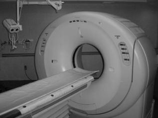
The gantry is the donut shaped main body of the computed tomography system and contains the x-ray source and detector system, as well as the mechanics for moving these devices as needed to perform the scan. The patient is extended on the table into the gantry aperture or hole in the gantry so that the X-ray source may rotate around the areas to be scanned (Fig. 6). The scannable region within the gantry is somewhat smaller than the gantry aperture or hole size. Typical is a 50 cm scan field of view within a 70 cm gantry aperture.
The entire gantry is usually pivoted to allow the top of the gantry to tilt toward or away from the table by 308 or more. This allows acquisition of images that are aligned or oriented to specific anatomy, such as the aligned with the disk in the lumbar spine. This feature is being used less, however, with the increasing use of thin slice data acquisition with MDCT systems permitting high quality computer generated images of alternate planes. The gantry also has localizer lights or lasers, and the table and gantry tilt controls to assist the technologist in posi-
Figure 6. The major system components in the scan room are the patient table, and the scanner gantry which houses the X-ray source, detector, and mechanical drive components.
tioning the patient. The mechanics within the gantry include a large turret bearing, larger than the gantry aperture, to permit rotation of the rotating components of the system, and motor drives and controllers to actuate the scanning motions. Slip rings and data transponders are used to transmit power and data between the stationary and rotating system components. The gantry may also include active or passive cooling devices to prevent heat buildup.
X-Ray Source
An X-ray tube and generator are needed to produce the radiation for the scan. In the X-ray tube a negatively charged hot filament or cathode emits electrons that are accelerated by a high voltage. The high energy electron strike a target that is part of the positively charged anode and produce X rays along with a considerable amount of heat. The X-ray technique is characterized by the specifying the tube current or mA and the tube voltage or kilovolts, which determine the amount and energy of the X-ray photons emitted. The generation of X rays is the same as is found in other radiographic imaging systems. A notable difference is the workload these tubes endure in clinical imaging. Consequently, the X-ray tubes in CT scanners are often the big-brother to the tubes found in general radiography, with a super-sized anode capable of holding the considerable heat developed during the scans. X-ray tubes designed for CT systems may have other features to prevent anode wobbling, which can cause artifacts, or to be more effective at removing the heat generated. Important parameters for the X-ray tube include its focal spot size, the heat capacity and the cooling rate of the anode. A small focal spot or X-ray source size can provide better image resolution, but a small size may limit the X-ray output that can be obtained. Since the X-ray tubes utilize a rotating anode, it is important that the axis of this anode is parallel to the axis of rotation of tube around the patient, otherwise considerable gyroscopic torque would be placed on the tube.
The X-ray generator includes the high voltage transformer used to create the high voltages necessary for X-ray production. A key requirement for CT systems is to have a highly stable voltage with little ripple or variation. Older systems often used bulky three-phase transformers and voltage rectifiers in order to produce a constant high voltage. Current systems tend to use high frequency sin- gle-phase generators. These systems take the utility supplied power and process it to produce a high frequency electrical source with frequencies typically in the range from 1000 to 2000 Hz. The higher frequency has several advantages. High voltage transformer efficiencies are much better at high frequency, and since it is single phase, only one pair of coils is required, making for a much smaller transformer package. Single-phase power is normally associated with 100% ripple as the voltage varies from zero to its peak value. At high frequencies, however, a minimal amount of capacitance in the system smoothes this voltage ripple to produce a nearly uniform voltage. This transition to high frequency transformers has been an enabling technology for helical scanning. In order to continuously rotate the tube around the patient, the high voltage X-ray power cables had to be eliminated. With helical imaging systems, a low voltage of a couple of hundred volts is transferred to the rotating portion of the gantry through an electrical slip ring. The high voltage transformer is mounted on the rotating portion and circles the patient along with the X-ray tube, thereby eliminating the constraint of a single rotation on the older systems. Even with the smaller and lighter generator package, there is considerable mass rotating around the patient, and considerable G forces on these components, especially with the subsecond rotation times.
Collimation and Beam Filtration
Since high energy X rays cannot readily be focused like light, a collimator blocks the X rays coming from the X-ray tube that are not directed at the detector. The X-ray beam is shaped by tungsten or lead plates into its fan beam shape. The width of the fan beam may be varied allowing the technologist to select the slice thickness. On single slice CT scanners, with a single linear array of detectors, the tube side collimation determines the slice thickness. On MDCT systems, the width of the detector or the averaged grouping of detectors determines the slice width. The nominal slice width or thickness is the thickness of the reconstructed voxel at the center of the scanner.
Additional X-ray beam filtration is also in the X-ray beam. Beam filtration is material the X rays pass through before getting to the patient. Legally a certain amount of filtration is required in order to remove the soft or low energy X rays that contribute significantly to the patient dose with little chance of passing through the patient contribute to the transmitted signal. The CT scanner beams are generally heavily filtered, not only to reduce patient dose, but it also reduces beam-hardening artifacts. Most scanners also utilize a bowtie or compensating X-ray filter. This is a filter that has a variable thickness along the length of the fan beam, being thinner at the center of the field and thicker toward the edges of the scan field, thus
COMPUTED TOMOGRAPHY |
235 |
Figure 7. The X-ray beam is filtered to reduce the low energy X rays, passes through a bowtie shaped compensating filter that reduces peripheral dose to the patient, passes through the patient to the radiation detector array.
looking like a bowtie. This filter helps reduce the peripheral dose to the patient and also can help reduce beam hardening variations by adding attenuating material to the portions of the beam that are going through thinner portions of the patient (Fig. 7).
X-Ray Detector and Data Acquisition System
The X-ray detector is a critical component of the scanner system. It should be efficient at absorbing the X-ray beam energy, and converting the X rays into the detected signal, and should have a rapid response time to allow for rapid data acquisition. The detector size, along with the X-ray tube focal spot size, limits the potential image resolution (22).
Scintillation Detectors. The detector found in Hounsfield’s original scanner was a sodium iodide (NaI) scintillation crystal linked to a photomultiplier tube (PMT). These types of devices are commonly used in nuclear medicine counting systems. The X rays are absorbed in the scintillation crystal where they are converted into a number of light photons. The PMT is a very sensitive detector of light and measures the light output. In nuclear medicine counting, the number of high energy photons entering the scintillation crystal is limited and each photon is analyzed and counted separately. With X-ray systems the rate at which photons are entering the detector is much faster than the ability of the system to detect separate distinguishable scintillations or flashes of light. The CT scintillation detectors are operated in a current mode rather than a pulse mode and measure the overall intensity of light produced instead of individual pulses of light.
A number of different scintillating or fluorescent materials have been used in CT scanners including cesium iodide (CsI), cadmium tungstate (CdWO4), and fluorescing materials using rare earth elements, such as gadolinium and ytterbium. Important characteristics of the detector material include its X-ray absorption efficiency, the energy conversion efficiency, and its temporal response. The X-ray absorption efficiency depends on the density and atomic
236 COMPUTED TOMOGRAPHY
number of the material, as well as the thickness of the detector. Conversion efficiency is the ability of the fluorescing material to take the energy that is absorbed and convert it to light that can be measured by the light sensitive detectors. When the X ray is absorbed the light is emitted over a short period of time. If this time to emit the light is too long, then this afterglow may influence subsequent measurement. This is one of the reasons that NaI(Tl) is not used in current fast scanners.
Additional factors affecting the detector efficiency is the effectiveness of getting the produced light to the light detecting element and the efficiency of this light detector. The photomultiplier tubes of early scanners have been replaced by photodiode arrays. These components do not have the inherent amplification found in PMTs, but they enable the manufacture of small, closely spaced detectors and the implementation of 2D or multirow arrays.
Gas-Filled Detectors. Gas-filled ionization detectors are another type of detector system that was widely used in CT systems. These detectors operated on the principle that the X rays passing through matter, such as the gas in the detector, causes ionizations or free electrons. A voltage can be placed across the gas to collect the electrons and determine the number of ionizations and the amount of radiation. This type of detector is used in many X-ray survey meters. In order to increase the fraction of the radiation that interacted with the gas and increase the signal level, high pressure xenon gas is used. The electrodes are tungsten plates that are oriented toward the position of the X- ray source. This directional chamber limits the detector sensitivity to radiation coming at an angle from these tungsten plates, thereby providing a capability to reject some of the scatter radiation entering the detector. These systems have been supplanted by the solid-state, scintillation detector systems, especially with the advent of MDCT.
Multiple Row and Area Detectors. The scintillation material in the MDCT detectors is mounted onto a photodiode array chip. The scintillation crystal is diced or sawed to form a series of individual elements. The sawed surfaces, or with the assistance of a reflective coating, help direct the light produced to the light sensitive component directly beneath this element. The width of the
detector, in the slice thickness |
direction, is |
typically |
0.5 mm. The number of rows |
of data that |
may be |
acquired is often limited by the data acquisition system (DAS). The signal from a series of rows may be combined to produce an effective slice thickness that is some multiple of this value. This may be done prior to the digitization, allowing for a thicker slab of tissue to be scanned per rotation, or may be done as a postprocessing technique to reduce image noise.
An example may be a four slice CT scanner with a series of 1.0 mm detector rows covering a total width of 20 mm. It is limited to acquiring four rows of data by its data acquisition system. A scan may be performed with 4 1 mm detectors for a total beam width of 4 mm, or 4 2 mm for a beam width of 8 mm, up to a 4 5 mm for a beam width of 20 mm (Fig. 8). The first approach would give the best interslice resolution, while the latter would allow one to scan a given volume in less time.
The DAS must provide a highly accurate digitization of the signal and is handling a tremendous amount of data. As an example a 64-slice scanner may have 64-active rows of detectors each containing 1000 elements. As the scanner rotates around the patient in 0.5 s, 1000 measurements are made from each of these elements. That results in 128 million precision measurements made each second. This value increases as more rows of detectors are added and area array detectors for cone beam scanning are used. Data acquired during the scan is transmitted by a telemetry system to the fixed portion of the gantry. The data is sent to a computer that utilizes array processors for rapid data
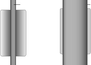
Figure 8. (a) In a single slice CT scanner the entire width of the detector is active and the slice width is determined by the collimated width of the X-ray beam.
(b) Multidetector CT slice width is determined by the effective detector width. Individual detector elements may be grouped to yield a larger effective slice thickness. In this example a detector array consists of 20 rows each 1 mm wide. A four slice CT system may use groupings of four rows yielding 4 rows of 4 mm wide detectors as shown, or can use other groupings of the 20 rows.
Single slice detector array |
Multi-slice detector array |
|||||||||||||||||||||||
|
X-ray beam |
|
|
|
|
|
|
|
|
|
|
|
|
|
|
|
|
|
|
|
|
|
X-ray beam |
|
|
|
|
|
|
|
|
|
|
|
|
|
|
|
|
|
|
|
|
|
|
|
|
|
|
|
|
|
|
|
|
|
|
|
|
|
|
|
|
|
|
|
|
|
|
|
|
|
|
|
|
|
|
|
|
|
|
|
|
|
|
|
|
|
|
|
|
|
|
|
|
|
|
|
|
|
|
|
|
|
|
|
|
|
|
|
|
|
|
|
|
|
|
|
|
|
|
|
|
|
|
|
|
|
|
|
|
|
|
|
|
|
|
|
|
|
|
|
|
|
|
|
|
|
|
|
|
|
|
|
|
|
|
|
|
|
|
|
|
|
|
|
|
|
|
|
|
|
|
|
|
|
|
|
|
|
|
|
|
|
|
|
|
|
|
|
|
|
|
|
|
|
|
|
|
|
|
|
|
|
|
|
|
|
|
|
|
|
|
|
|
|
|
|
|
|
|
|
|
|
|
|
|
|
|
|
|
|
|
|
|
|
|
|
|
|
|
|
|
|
|
|
|
|
|
|
|
|
|
|
|
|
|
|
|
|
|
|
|
|
|
|
|
|
|
|
|
|
|
|
|
|
|
|
|
|
|
|
|
|
|
|
|
|
|
|
|
|
|
|
|
|
|
|
|
|
|
|
|
|
|
|
|
|
|
|
|
|
|
|
|
|
|
|
|
|
|
|
|
|
|
|
|
|
|
|
|
|
|
|
|
|
|
|
|
|
|
|
|
|
|
|
|
|
|
|
|
|
|
|
|
|
|
|
|
|
|
|
|
|
|
|
|
|
|
|
|
|
|
|
|
|
|
|
|
|
|
|
|
|
|
|
|
|
|
|
|
|
|
|
|
|
|
|
|
|
|
|
|
|
|
|
|
|
|
|
|
|
|
|
|
|
|
|
|
|
|
|
|
|
|
|
|
|
|
|
|
|
|
|
|
|
|
|
|
|
|
|
|
|
|
|
|
|
|
|
|
|
|
|
|
|
|
|
|
|
|
|
|
|
|
|
|
|
|
|
|
|
|
|
|
|
|
|
|
|
|
|
|
|
|
|
|
|
|
|
|
|
|
|
|
|
|
|
|
|
|
|
|
|
|
|
|
|
|
|
|
|
|
|
|
|
|
|
|
|
|
|
|
|
|
|
|
|
|
|
|
|
|
|
|
|
|
|
|
|
|
|
|
|
|
|
|
|
|
|
|
|
|
|
|
|
|
|
|
|
|
|
|
|
|
|
|
|
|
|
|
|
|
|
|
|
|
|
|
|
|
|
|
|
|
|
|
|
|
|
|
|
|
|
|
|
|
|
|
|
|
|
|
|
|
|
|
|
|
|
|
|
|
|
|
|
|
|
|
|
|
|
|
|
One 3 mm slice |
Four 4 mm slices |
Determined by x-ray beam collination |
16 mm collimated x-ray beam |

reconstruction, and manages the storage and display of the resultant images.
Computer and Operator Console
The operator console utilizes an interactive computer display and dedicated function buttons to allow the procedure setup, scan initiation, image display, and data storage. The demographic information for the patient may be received from the facilities radiology or hospital information system (RIS or HIS) or entered by the technologist. Editable routine scan protocols facilitate scan setup and preview radiographic type image is used to identify the specific volume of the patient to be scanned. The images are displayed and some image processing and measurement features are available. A limited amount of the raw transmission data is stored on the system and may be used to for additional reconstructions from the data with alternate parameters. The reconstructed images may be filmed and the image data archived on the scan computer system, or transferred to a central PACS system for storage and for remote image display.
SCAN PITCH AND EFFECT ON PATIENT DOSE
One of the technique parameters set when performing a helical scan is the scan pitch, which is like the pitch on a screw. This refers to the ratio of the distance the table moves per 3608 rotation of the X-ray source to the thickness of the X-ray beam. If the table moves the same distance as the beam width each rotation, then the scan pitch is one. The radiation dose with a pitch of one is similar to that obtained in a step-and-shoot axial mode where the table incrementation between scans equals the slice or beam thickness. With these contiguous axial images the entire surface of the patient within the area scan is struck once with the primary, unattenuated X-ray beam. Having a pitch < 1 indicates that overlapping data is acquired with a commensurate higher average dose, and a pitch greater than one results in gaps between primary exposed areas and a lower average radiation dose. A pitch < 1 requires less data interpolation and yields sharper slice profiles, while pitch > 1 reduces dose, but may blur the slice thickness profile and is more subject to certain image artifacts. With some CT systems this change in the effective technique and average dose as a result of the selected pitch is reported as the effective mAs. The effective mAs is the X-ray tube current (mA) times the time per rotation divided by the pitch.
The concept of pitch gets a little more complicated with MDCT systems. With single-slice CT systems the slice thickness corresponded to the detector width. In MDCT systems, there are multiple rows of detectors covering the width of the X-ray beam. This leads to two separate, but related pitch values. There is the collimator pitch that relates the table motion to the overall X-ray beam width, and the detector pitch that relates the table motion to the width of the individual detector rows (or their combined width when rows are combined prior to digitization) (23).
Consider an example with the four slice scanner with 20 rows of 1.0 mm wide detectors described above with a scan
COMPUTED TOMOGRAPHY |
237 |
time per 3608 tube rotation of 1 s. If the data acquisition mode is 4 2 mm, that is to simultaneously acquire four sets of data from detectors having a detector width of 2 mm, then four pairs of 1.0 mm physical detectors will be combined to produce four detector rows each with an effective 2 mm detector width, and the overall collimated beam width is 4 2 mm or 8 mm. If the table incrementation speed is 6 mm s 1 or 6 mm/rotation, then the collimated pitch is
Collimator pitch ¼ |
Table travel per tube rotation |
ð1Þ |
|||||
|
|
|
|||||
|
Collimated beam width |
||||||
Collimator pitch |
|
|
|
|
|
||
|
Table travel per tube rotation |
|
|||||
|
|
|
|
|
|
|
2 |
¼ Number of detector rows |
|
Detector width |
|||||
|
ð Þ |
||||||
Collimator pitch ¼ |
6 mm=rotation |
||||||
4 2 mm |
|
|
|
|
|||
Collimator pitch ¼ 0:75
A collimator pitch < 1 indicates that the radiation fields are overlapping, which will result in a patient radiation dose higher than an equivalent set of contiguous slices or a pitch of one. The detector pitch in this example is given by
Detector pitch ¼ Table travel per tube rotation Detector width
6 mm=rotation ð3Þ Detector pitch ¼ 2 mm detector width
Detector pitch ¼ 3
CT SCAN TECHNIQUES
Preview Digital Radiograph
There are several scan modes or types of data acquisition that a CT scanner may be to acquire data. One commonly used technique is the acquisition of a scout or preview scan. These scans are basically a digital radiographs that are used to set up the tomographic imaging sequence, or may be used to visually locate the position of an axial slice on a radiographic reference image. To acquire the preview image the X-ray source and detector remain stationary. The detector sees a single line of an X-ray transmission image. As the table and patient are moved through the X-ray fan beam, the series of transmission lines acquired generate the radiographic image.
From the preview scan the technologist can define a range or volume within the patient to be scanned. Lateral preview scans can be used to determine the proper gantry angulation to orient the tomographic slices with desired anatomical structures, such as to the intervertebral disks in the spine.
Axial CT Scan
An axial scan is a basic CT scan, normally implying the data being acquired without the table moving during data

238 COMPUTED TOMOGRAPHY
acquisition (Although an axial image also refers to any image orientated transverse across the patient, as opposed to sagittal or coronal plane orientations.) Prior to the advent of the continuously rotating helical scanners, all CT scans were acquired with a stationary table. For a single-slice scanner the slice thickness or slice profile is defined by the collimation of the X-ray beam with the detector width being somewhat larger than this beam. For a multidetector CT the effective detector width of the rows of detectors tends to be the primary factor in determining the slice thickness. The effective detector width may be the summation of several physical rows of detectors. The grouping of detector rows may be to form thicker slices in order to reduce the image noise and number of images generated, or may be due to data acquisition system limitations.
The MDCT systems may be limited in their ability to acquire axial images due to the divergence of the fan beam. With a single detector row all of the transmission rays passed through a particular plane within the patient. The beam divergence along the slice thickness orientation caused some variation in the detected slice profile, but it was relatively minor. With the MDCT systems the data seen by the row of detectors on the ends is not consistently within a single plane due to the angulation of the diverging X-ray beam. This can cause inconsistencies in the data and may cause image artifacts or errors.
Helical CT Scan
The primary advantage to the continuously rotating source and detector is the ability to do helical or spiral CT scanning. Data is acquired as the patient is moved through the beam. There is no set of measurements where one has transmission data from all angles around the patient, but adjacent measurements are used to estimate the data corresponding to a particular plane. This mode allows for the rapid acquisition of data though a patient, and the ability to reconstruct images at any location within this volume. This rapid scanning allows procedures to be done quicker, often allows data to be acquired within a single breathhold, minimizing motion blurring, and facilitates the ability to perform contrast enhanced angiography studies to evaluate major blood vessels.
Dynamic Scan, Fluoro CT, and Triggered Scan Start
Another mode of data acquisition is dynamic scanning. In this mode a series of images are sequentially obtained at a single location. This can be used to analyze motion, or more commonly to evaluate the flow of contrast material into a tissue. This capability prior to continuously rotating systems was limited to one scan every few seconds since the tube had to stop and reverse motion between scans. Continuously rotating systems not only can acquire a sequence of images with no time gap between them, but also can obtain images overlapping in time where the time spacing between images is shorter than the data acquisition time for the image. Dynamic scanning can produce a series of images to assist in evaluating a tumor or mass by how it enhances or changes as iodine contrast material flows into
the tissue, or it may be used for quantitative analysis of the tissue perfusion.
A variation of this is fluoro or fluoroscopy mode CT. Here a series of images at a location are dynamically scanned and rapidly reconstructed to allow the technologist or physician to see the image in real time. This may be used to assist in a CT guided invasive procedure. Note that another approach is to have a conventional X-ray fluoroscopy system adjacent to the CT where the fluoroscopy is used for needle or catheter guidance and the CT is used to verify and evaluate results. Computed tomography fluoroscopy may also be used to visualize the arrival of injected contrast material into a vessel. This information may be used to initiate a scan sequence to catch the maximum concentration of the contrast media in the vessels of interest for CT angiography. Angiography scan starts may also be assisted using a feature where the computer evaluates the transmission data through a defined vessel and triggers scan start when a sufficient attenuation increase is detected.
Cardiac Gated CT
Physiologic motion can degrade the image quality. Fast helical and MDCT techniques allow for single breathhold studies. With the exception of the electron beam CT systems, a full set of data cannot be acquired of the heart without motion. In order to freeze the cardiac motion, the data is acquired and characterized relative to the cardiac cycle and is selectively grouped to obtain images without the typical motion blurring. This gated imaging requires an electrocardiogram (EKG) or similar input from the patient to define the cardiac cycle (24). Since the heart is relatively stationary during the longer diastolic rest phase than during systolic contraction, the gating may also be used to eliminate or minimize the systolic data to produce a diastolic only image. Alternatively, data can be acquired over many cardiac cycles and binned to produce images for various portions of the cardiac cycle. This multi-phase imaging process is similar to what is done in gated nuclear medicine and MRI studies. The series of images may be viewed in a movie mode to visualize the beating heart, and may be analyzed regarding wall motion and cardiac output.
CT NUMBERS
The linear attenuation coefficient is scaled into an integer pixel value. Medical systems utilize an offset scale that is normalized to water. This scale assigns air a CT value of
–1000, water is at 0 and a material twice as attenuative as water has a CT value of þ1000, and so on. The CT number is an integer relating to the attenuation properties of the tissue by the following formula.
CT number ¼ ðmtissue mwaterÞ 1000
mwater
Where mtissue and mwater are the linear attenuation coefficients for the tissue in the particular voxel, and of water,
respectively. Typical CT number values for some common tissues and test objects are listed in Table 1.
Display Window and Level
The CT numbers are commonly stored in the computer as 12 bit integers covering a CT number range from 1000 to þ3000 (or 1023 to 3072). To display the full possible range of data one needs > 4000 shades of gray or displayed intensity. The human visual system, however, is limited, and we generally can discern something closer to 30 different shades. A common technique with all of the digital imaging methods is to use a viewer selectable mapping of the digital numbers representing the image to the various displayable intensities. There are a number of variations and processing methods that can be applied, but one of the most basic and most used methods is to define a display window level and window width.
The window level value defines the CT value that will be mapped as the middle gray intensity. The window width is the range of CT numbers that will have a range of gray values from black to white. Everything below the lower range value (the window level minus one-half of the window width) will be black and everything above the upper range level (the window level plus one-half of the window width) will be white. By adjusting these levels one can ignore the air-like CT densities, and display all the dense structures, such as bone as white, while obtaining a relatively high contrast view of the a narrow range of CT numbers corresponding to the soft tissue densities within the body. On the computer display one can easily vary these settings to look at low density structures in the lung or the high density detail of the bone if desired. Example of the effect of display window settings on the displayed image is seen in Fig. 9.
Other variations to this gray scale mapping function can also be performed, such as histogram equalization, where the resultant display will have an equal number of pixels for each gray level. The display may also be done in color where each CT number is mapped to a particular color. This is sometimes referred to as psuedo-color to emphasize that the displayed color is not that of the object, but some arbitrary assigned color. Clinical CT generally does not use color for basic cross-sectional image viewing. Color is commonly used, however, for processed data displays, such as 3D surface imaging where one views the surface of organ structures or of the vascular tree, or may be used as an overlay over the gray scale anatomical image with the color representing some functional feature, such as blood perfusion.
DISPLAY TECHNIQUES
Film and Soft-Read Workstations
Traditionally the cross-sectional images generated in a clinical procedure are windowed as appropriate for the tissues of interest, and then photographed or printed onto a large 14 17 in. (356 531 mm) transparent film. If necessary, two sets of films may be made to have the window level and width adjusted for two different CT number ranges, such as for soft tissue and for the lower densities within the lung. The films provided a highly portable record of the study that can be illuminated with
COMPUTED TOMOGRAPHY |
239 |
any X-ray film viewbox, and provides a medical record of the procedure. This was a manageable process producing a handful of films when used with single slice scanners acquiring relatively thick slices (3–10 mm) through a volume of interest.
With the fast MDCT systems one can rapidly scan through the same volume of the patient with thin slices. This results in hundreds to thousands of images for a single procedure. This would result in many dozens of films per study, which is not only expensive, but also unwieldy for physician review. This has been one of the drivers to implement a picture archiving and communication system (PACS) (see PACS topical entry), which enables the use of computerized soft-read workstations for the primary analysis of the image set.
Analyzing the images from the computer display provides a number of interactive tools for the reviewer. The ability to interactively change the window level and width is a powerful function for evaluating subtle features. One can measure the area and average CT number within a region-of-interest (ROI), measure distances and angles, and magnify regions of the image. One can rapidly page through a stack of images providing a better view of the continuity of structures from slice-to-slice.
Alternative Image Plane Display
A number of processing techniques are available for analyzing and presenting the volume information contained in a stack of axial slices (Fig. 10a). An alternative plane through the patient can be generated through this volume. This can be a coronal (frontal) plane, a sagittal (lateral) plane (Fig. 10b and c), or an arbitrary oblique plane. A series of parallel oblique planes may be reconstructed in a batch mode using the multi-planar reformation feature of the scanner or workstation, or the location may be interactively defined and displayed. The reformatted slice may be generated with a definable slice thickness down to the voxel size of the data set.
Maximum Intensity Projection
The displayed data in the oblique plane display is an average of the voxels contributing to each of the reformatted pixels. An alternative is to display an intensity value that corresponds with the largest voxel value in these contributing pixels. This type of display is referred to as maximum intensity projection (MIP). The slab thickness for the MIP image can include the entire volume scanned or a thinner slab (Fig. 10d). The MIP image gives a 3D type presentation for viewing dense structures such as bone or contrasted blood vessels, especially when rotating the viewing angle.
3D Surface Imaging
Another volume viewing technique is the 3D surface imaging. If structures can be characterized by their CT number range, the contours of the structure can be defined and surface view formed. These images have much in common with the visualization techniques used by computer-aided design or in computerized animation in the entertainment

240 COMPUTED TOMOGRAPHY
Figure 9. Various display window width and window level settings for the same abdominal CT image. (a) A wide window (2000 CT numbers) shows nearly the full range of CT numbers, but without discernable contrast between soft tissue structures. (b) A narrow window (WW ¼ 150) yields high contrast between structures, but the window level centered at 150 results in most soft tissue being black because they are below the window range, with only the bone and structures containing iodine contrast media being seen. (c) A narrow window (WW ¼ 150) centered at 50 results in a high contrast visualization of the soft tissue. (d) A typical display window (WW ¼ 500, WL ¼ 100) may compromise to provide good contrast while displaying a wider range of structures with lower displayed noise.
industry. The surface defining points are connected and plated with tiles or surface segments (25). The display software will project the nearest surfaces to the displayed image and use features such as distance from the viewer
and angulation of the surface to define the brightness intensity. Light source position and coloration may also add to the display. Several different structures with differing CT number ranges can be simultaneously displayed

with different color schemes for each structure. In this way, bone may be shades of white while a tissue or vascular structure may be red (Fig. 10e and f). The structure may also be given the property of transparency allowing visualization of deeper features, such as visualizing the ventricles of the brain through a visible but transparent skull. With specialized displays a stereoscopic pair of images may be viewed, enhancing the 3D effect, however, the ability to use motion and rotate the structures on the display is very effective at producing a 3D view.
COMPUTED TOMOGRAPHY |
241 |
Three-dimensional views may be enhanced with some computerized surgery. The user can select certain structures to be eliminated from the image. This selection can be made by defining cut planes or surfaces from various views and erasing structures outside of a volume of interest. Connectivity tools may also be used where the cursor is used to identify a structure, and then all surface points that are contiguously connected to the seed point are either selected or erased. In this way, one may select a vascular tree that is otherwise obscured by bony structures with
242 COMPUTED TOMOGRAPHY
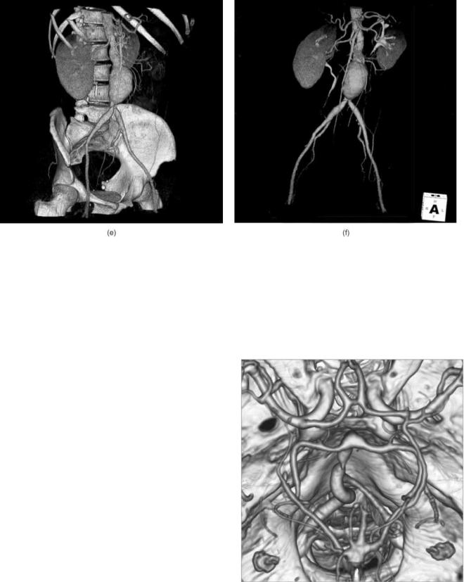
Figure 10. Alternative image sets can be generated from a series of closely spaced axial images. The image in (a) is one of 266 2.5 mm thick axial images. Iodine contrast media has been injected into the patient to make the major blood vessels visible, including the balloon shaped aortic aneurysm. From this data set the computer can generate (b) a sagittal image, or (c) a coronal image, or
(d) a maximum intensity projection (MIP) image of a sagittal slab containing the spine and aneurysm. Structures may be identified by their CT number range to generate 3D surface images of bone and contrasted vessels (e), and structures may be removed to produce a vascular tree image.
similar CT numbers. Problems with this approach occur when the two structures touch making a connectivity bridge between them.
SPECIAL CLINICAL FUNCTIONS
Surgical Planning
The ability to produce a 3D visualization of structure surfaces can be used in several ways. It is useful for general viewing and obtaining an overview of certain structures. This may be useful in seeing areas that should be scrutinized more closely, and appears useful in communicating anatomical findings to surgeons and other physicians that are more familiar with the physical anatomy rather than a series of cross-sectional slices through it. In some cases data may be obtained from these images to assist in surgical planning, including the repositioning of bone fragments or the appropriate type and size prosthetic hardware to use.
CT Angiography, Virtual Colonoscopy, and CT Perfusion
Imaging
Computed tomography angiography (CTA) is the procedure used to visualizing the blood vessels (26–28). Iodine contrast media is injected into the patient to increase the attenuation and increase the CT number of the blood within the vessels (Figs. 10e, f, and 11). Timing of the
Figure 11. Three-dimensional view of a CT angiogram of the brain arteries including the Circle of Willis along with the skull structures as viewed from the top of the head.
CT scans is important in these procedures since the contrast media will return through the venous system and obscure the visualization of the arterial system, hence the use of some of the previously described scan start techniques. Besides general 3D viewing of a vascular tree to produce a CTA, other related techniques may provide additional information. Two points in a vascular tree may be identified and the computer can locate the line within the scan volume corresponding to the center of the vessels connecting them. The vessel along this line may be analyzed producing a plot of the vessel diameter or cross-sectional area. A stenosis appears as a reduce area, while an aneurysm may be seen as a greatly enlarged area. Since the vessel wall is defined as the surface between the high X-ray densities within the vessel to the water-like tissue densities outside the vessel, one can use 3D visualization techniques with the viewer located inside of the vessel. The viewer may travel or fly-through the vessel and visualize the structure of the lumen surface.
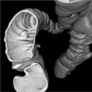
This fly-through technique is also the basis of virtual colonoscopy. In a clinical colonoscopy, the bowel is prepped to remove residual feces. An endoscope is inserted into through the anus into the colon and a camera and light source allows visualization of intestinal surface. If suspicious polyps or lesions are located, devices may be guided through the endoscope to remove or sample the tissue. In virtual colonoscopy bowel preparation is still needed and the colon inflated with air to produce a well-defined interface at the wall surface. A series of CT slices are acquired and 3D visualization and fly-through techniques are used to view the structure of the colon surface (Fig. 12).
Besides visualizing the vessel by CTA, the vascular condition of the tissue may be analyzed using a CT
Figure 12. A 3D surface image of the interior wall of the colon allows a virtual colonoscopy fly-through to inspect the intestinal wall for polyps.
COMPUTED TOMOGRAPHY |
243 |
perfusion procedure, especially in evaluating the brain. Acquiring the data in a perfusion study requires obtaining a series of images of selected slices over a short period of time as iodine contrast media or inhaled xenon gas in the blood flows into and washes out of the tissue. Various parameters may be measured, such as mean transit time (MTT) showing how fast the blood reaches the tissue. This may provide some indication of blood shunting or obstruction. The enhancement curve may be analyzed to obtain a relative cerebral blood volume (rCBV) and relative cerebral blood flow (rCBF) images. This information may be useful in evaluating strokes and obstructive disease.
Quantitative Analysis: Bone Density and Calcium Scoring
In general clinical CT scanners are not designed to produce highly accurate attenuation data, but rather high quality diagnostic images with minimal artifact. A number of factors can affect the calculated CT number value within a pixel, including its location and the size of the patient. With this caution, however, there are several applications where the analysis of the CT numbers is valuable. In general image interpretation, the CT value of a tissue lesion may be made to help determine if it is a mass, a cyst, edema, or a hemorrhage. Other scans may be performed specifically for the quantitative analysis. One screening procedure is calcium scoring. The calcium plaques in blood vessels will increase the CT value of the corresponding pixels. An evaluation of the amount of calcium in coronary arteries is an indicator of cardiac risk and may be measured by CT (29).
Osteoporosis is the loss of calcium bone mass, especially prevalent in postmenopausal women. The CT technique may be used to analyze the calcium content of the bone. Usually the trabecular bone in the middle of the spinal vertebra is analyzed due to their large surface area and sensitivity to bone loss. In order to produce reproducible data, the measurements made of the bone are compared to other reference densities within the image or in a comparable image. This may be done by having the patient lie on a phantom containing known reference materials, or comparing the measurements to other tissue in the image with known CT values (30–32). Most bone mineral densitometry, however, is performed with dedicated systems rather than using CT scan procedures.
Radiation Therapy Treatment Planning
Another group that would like quantitative information is the radiation oncologist for use in radiation therapy treatment planning. Some CT scanners are dedicated for radiation oncology use and these CT simulators may have special features and software to assist in radiation therapy simulation. In radiation therapy treatment planning it is important to be able to define the target tissue to be irradiated and the adjacent sensitive tissues, and to have them in the same position and orientation that they will be at the time of treatment. Since most linear accelerators used for treatment have flat tables, a hard flat table pad should be used for the corresponding CT scan. Likewise the body position, such as the position of the arms, should be as
244 COMPUTED TOMOGRAPHY
it will be during treatment. Skin markers and CT visible fiducial markers may be used to orient and register the images with the treatment plan.
Besides seeing the pathology and anatomy to identify the targets for the treatment planning, obtaining information on the attenuating properties of the various tissues to the high energy photon and electron beams is useful for accurate treatment planning. The problem is that diagnostic CT scans are acquired at relatively low photon energies as compared to that used in therapy. The diagnostic CT X-rays are much more sensitive to the atomic number of the materials within the voxels than are the high energy therapy beams. Characteristics of known tissues are used along with the measured CT numbers to estimate the physical or electron density of the tissue and its high energy attenuating properties.
Dual-Energy Scanning
One approach that can be used for quantitative imaging, in particular to determine effective atomic number and density of the tissue is dual energy scanning. Using two different X-ray beams will produce data corresponding to the attenuating properties at the two separate effective energies. At diagnostic X-ray energies the primary attenuation processes are photoelectric absorption and Compton scattering. Photoelectric absorption is highly dependent on the atomic number of the material and the probability of interaction falls off rapidly with increasing photon energy. Compton scattering is relatively independent of the atomic number and falls off at a much slower rate. That is, the probability of photoelectric absorption is proportional to Z3/E3, while Compton scattering falls off with 1/E. This information may be used to take the CT measurements and calculate an alternate pair of basis images, such as effective atomic number and density (33). This is preferably done with the transmission data, but may be performed with the reconstructed images. Challenges exist in these calculations, however, due to other factors in the imaging process, and methods used to correct for other systemic errors.
Stereotactic Surgery Planning
Stereotactic surgery utilizes a hard fixed frame to the head to direct a needle to a very particular location in the brain. The base frame usually is attached to the skull with screws or pins. During CT scanning a localizing frame is attached to the base. When the CT scans are analyzed, the target location is identified in the images. The location of various frame components are also identified and recorded. This information is used to localize the target in the 3D frame space. During the surgical procedure the localizing frame is replaced with a needle guide that can be set for insertion to the target spot. The same approach is used for stereotactic radiosurgery where thin radiation therapy beams are used to irradiate specific targets in the brain.
PET–CT Image Fusion and PET-CT Scanners
Positron emission tomography (PET) scanning is a specialized nuclear medicine technique for generating
cross-sectional images of the distribution of positron emitting radioactive tracers in the body. In this task, it is very sensitive at presenting this information. It is, however, relatively poor at presenting high resolution detailed anatomy. The PET images may be fused with corresponding CT images to delineate the structures containing the radioactive tracer. This is usually displayed as a color PET image overlaid onto a grayscale CT image. The alignment of the two data sets may be performed manually or automatically by various computer algorithms. A key aspect of this image fusion is the patient being in identical positions for both data sets. This can present problems including different table shapes, arm position, flexure of neck and back, or changes in the patient between the scans.
Much of the difficulties in image fusion are eliminated by the use of a specialized system that contains both the PET scan capability and CT scan capability (34,35). Typically these are two relatively independent scanners with a connected gantry and utilizing a single patient table system. One of the steps in PET scanning is to acquire transmission measurements through the patient in order to perform accurate attenuation correction of the data. On a stand-alone PET scanner, this is acquired by use of a radioactive source that emits similar photon energies. With PET–CT the CT image data may be used to determine the PET attenuation correction. Note that the CT scan represents X-ray attenuation properties at diagnostic X-ray energies, which are much lower than the 0.511 MeV photons from the PET radionuclides, and appropriate corrections must be applied.
RADIATION DOSE
Computed tomography is an X-ray procedure with an associated radiation dose. X rays are ionizing radiation, meaning that the X-ray photons have sufficient energy to rip orbital electrons from atoms. As a consequence, small amounts of absorbed energy can cause biochemical actions that may have biological consequences. Radiation dose is the amount of energy absorbed per mass of tissue at a defined location and is measured in rads or preferably in the SI unit of grays, where
1 Gy ¼ 1 J kg 1 ¼ 100 rads |
ð4Þ |
Related are units of effective dose, the rem and sievert, which estimate the whole-body dose that has an equivalent long-term risk as an actual dose to just part of the body (36). Risk from radiation exposure can be divided into a couple of categories. Nonstochastic or deterministic effects are those that will happen if a certain radiation dose is received. Most relevant to diagnostic imaging are skin effects, such as erythema, the reddening of the skin. These effects require several gray of dose, which is significantly higher than doses normally encountered in CT. Stochastic or statistical biological effects are of some concern and should be part of the risk–reward evaluation for the procedure. The principal stochastic effect is the increase risk of getting cancer as a consequence of the radiation exposure. The risks are relatively small, but
unwarranted radiation exposures should be avoided. Since developing embryos and fetuses are especially sensitive to radiation, special cautions are often taken to minimize in utero exposures.
Computed tomography is a bit different from standard radiographs relative to the total dose received. The maximum entrance dose to the skin may be quite similar between a CT scan and a radiograph, but in radiography the intensity of the radiation decreases due to attenuation as it passes through the patient. Consequently, the dose to deep structures is much less than the surface dose, and the dose at the exit surface can be orders of magnitude less than the entrance dose (37,38).
In CT, the X-ray source rotates around the patient, such that the entrance surface is not just on one side of the patient. This results in a more uniform dose and considerably more total energy deposited in the patient. In a typical head scan, the dose across the imaged slices is fairly uniform, and for body sections the midline dose is approximately half that of the surface dose. This results in a much higher effective dose to the patient. It is estimated that CT accounts for 10% of the radiology imaging procedures, but amounts to around two-thirds of the total effective dose patients receive, and these values are likely to increase with the increasing utilization of CT.
Measuring radiation dose in CT presents some challenges. The X-ray beam is a narrow fan beam and may not even be constant across its width. Bow-tie compensating filters may further vary the beam intensity along the length of the fan beam. We see that slice width and spacing, and helical scan pitch, as well as the patient size, are also factors affecting the average dose.
Dose across the slice thickness, either in air or within a plastic phantom that simulates the patient, may be measured with a stack of thermoluminescent dosimeter (TLD) chips, with a radiation sensitive dosimetry film, or with a photoluminescent dosimeter strip. This data can be useful in characterizing the dose profile and the amount of scatter radiation present. Acquiring this data is cumbersome, and the use of this information to estimate a dose from a series of scans can be complex.
An alternative is to measure the CT dose index or CTDI. If one considers a series of contiguous slices, where the distance between the centers of adjacent slices is equal to the slice thickness, then the dose to a particular point in the patient is equal to the primary dose from the slice containing that point, plus the scatter radiation from the other slices. The CTDI is effectively this multiple slice average dose. It is measured with a long thin cylindrical chamber, typically 100 or 140 mm in length, about the size and shape of a pencil. It is exposed with a single axial scan. If the slice thickness is 5 mm, then the center 5 mm of the chamber receives the primary exposure. The adjacent 5 mm segments encounter the exposure for the adjacent slices, and the next 5 mm the scatter dose two slices away, and so on for the full length of the chamber. If one normalizes the measurement for to the 5 mm primary segment length, the overall measurement is the exposure from the primary beam plus scatter this location would receive from CT scans of the surrounding slices. In general,
COMPUTED TOMOGRAPHY |
245 |
the CTDI is given by
CTDI ¼ ðmeasured exposureÞ ðf factorÞ
|
chamber length |
|
ð5Þ |
||
N |
|
slice thickness |
|
||
|
|
||||
The f-factor is the Roentgen exposure to the rad or gray dose conversion factor for the material being exposed. Alternatively, the ionization chamber measurement may be calibrated in air kerma or air dose and the appropriate air kerma to dose conversion factor for the material is used. The value N is the number of detector rows being used, and N times the slice thickness is the width of the X-ray beam. The ratio of chamber length to the beam width is one over the fraction of the chamber that is exposed with the primary beam.
The measurement of CTDI is a straightforward measurement with the proper equipment. The phantoms used to simulate the attenuation by the patient are typically acrylic cylinders with a diameter of 16 cm for the head phantom and a diameter of 32 cm for the body phantom. The phantom has a hole in the center and at four locations near the periphery of the phantom for insertion of the pencil shaped CTDI ionization chamber.
A composite measurement of the center and peripheral value is the weighted CTDI or CTDIw. It is given by
|
1 |
|
2 |
|
|
||
CTDIw ¼ |
|
CTDIcenter |
þ |
|
|
CTDIperipheral |
ð6Þ |
3 |
3 |
||||||
These CTDI values should correspond to the multiple slice average dose from a series of contiguous axial scans. This value should also correspond to the dose from an equivalent helical scan with a collimator pitch of one. If the axial slices overlap or the helical pitch is less than one, the dose will be higher. If the axial slices have gaps between them or the helical pitch is > 1, then the average dose will be lower. The volume CTDI or CTDIvol dose estimate adjusts the CTDIw for the slice spacing or pitch.
CTDIvol ¼ CTDIw
detector width number of detector rows table increment per 360 tube rotation
CTDIvol ¼ CTDIvolCTDIw ð7Þ pitchð7Þ
A number of factors affect the patient dose. Some are defined by the design of the scanner, such as tube to patient distance, and the X-ray beam filtration. The patient size affects the attenuation and the subsequent dose for a given technique. Others are selectable by the technologist, (e.g., the kVp, mA, rotation speed, and pitch or slice increment). Since the X-ray output is directly proportional to the tube current or mA, then the total output per rotation, hence the dose, is directly proportional to the mA and the time per rotation. The dose is also related to the tube accelerating voltage or kV, but proportional to the kV to a power of 3. Note that even though the dose goes up with kV, often some of the other dose factors can be reduced for comparable image quality, especially for large patients. The average patient dose is inversely proportional to the collimator pitch in helical (39). For comparable image quality, a thick-body section
246 COMPUTED TOMOGRAPHY
requires a higher X-ray technique than does a thin-body section since a larger percentage of the incident X-rays are absorbed. Techniques are typically reduced for pediatric cases due to the smaller body size and higher concern for radiation exposure. Instead of selecting one technique to be used for all slices, the scanner may have a type of dose modulation or automatic exposure control that reduces the mA for less attenuatingbodysections.Thismaybe performed based on data from the preview scan, or may be determined by the attenuation found in the previous rotation (40,41).
CT RECONSTRUCTION METHODS
There are several different reconstruction methods or mathematical algorithms that can be used to estimate the cross-sectional distribution of attenuation coefficients that results in the measured set of X-ray transmission values (5,6,39). Knowledge of the basic elements of the reconstruction method can help determine elements relating to the image quality, and artifacts. Reconstruction methods can be categorized into two basic approaches: analytic and iterative reconstruction techniques. The primary reconstruction method in medical CT systems is the filtered backprojection method, an analytic reconstruction technique.
Projection Data
What is the relationship between the measured transmission data and the CT data values? It is necessary to normalize the measured transmission data and convert these values into projection values that correspond to the objects attenuation values. The projection data values for a narrow, monoenergetic beam of X radiation can be determined by considering Lambert’s law of absorption
I ¼ I0e ms; |
or |
ð8Þ |
I=I0 ¼ e ms |
|
ð9Þ |
where I is the intensity of the transmitted beam, I0 is the initial intensity or intensity of the beam with no attenuating material present, m is the linear attenuation coefficient of the absorber material, and s is the thickness of the absorber. The linear attenuation coefficient corresponds to the fraction of the radiation beam that a thin absorber will absorb or scatter. This coefficient is dependent on the atomic number of materials present, the physical density, and the energy of the X-ray beam.
If instead of a single homogenous absorber there are a series of absorbers, each with thickness s, the overall transmitted intensity is
I=I0 ¼ e-m1s e m2s e m3s e m4s |
ð10Þ |
I=I0 ¼ eðm1þm2þm3þm4þ Þs |
ð11Þ |
I=I0 ¼ e Pmisi |
ð12Þ |
where mi is the linear attenuation coefficient of the ith absorber.
Considering a 2D section through an object of interest, the linear attenuation coefficients of the material distribu-
tion in this section can be represented by the function m(x,y), where x and y are the Cartesian coordinates specifying the location within the section. The integral equivalent to the above equation is then
R
I=I0 ¼ e mðx;yÞds ð13Þ
integrated along the line, s, from the X-ray source to the detector.
The objective of the reconstruction program in a CT system is to determine the distribution of m(x,y) from a series of intensity measurements through the section.
Inverting both sides of the equation to eliminate the negative sign, and taking the natural log of both sides to eliminate the exponential yields what is called the projection value, given by
Z
p ¼ lnðI0=IÞ ¼ mðx; yÞds |
ð14Þ |
This equation is the basis of the Radon transformation that is fundamental to the CT process. The inversion of this transform, going from the projection data to the 2D distribution was solved in 1917 by Radon (3). He showed that the distribution could be determined analytically from an infinite set of line integrals through the distribution.
The projection values are based on several assumptions that are not necessarily true in making practical measurements. This may require certain corrections to the data for these systemic errors, or may result in artifacts or degradations in the image. Some of these will be discussed relative to image quality and image artifacts.
Iterative Reconstruction Techniques
One of the broad categories of reconstruction is the iterative reconstruction techniques. With this approach an initial guess is made of the density distribution of the object. The computer then calculates the projection data values that would be measured for this assumed object in a process referred to as forward-projection. Each calculated value is compared to the corresponding measured projection data value, and the difference between these values is used to adjust the assumed density values along this ray path. This correction to the assumed distribution is applied successively for each measured ray. An iteration is completed when the image has been corrected along all measured rays, yielding an improved estimate of the object. The process is repeated and with each iteration the estimated object or reconstructed image improves its correspondence to the object distribution.
There are numerous variations of iterative processing that may be used. One of the most popular is the Algebraic Reconstruction Technique (7), or ART, which in itself is an offshoot of the Kaczmarz technique for inverting large illconditioned matrices (42). The variations include additive or multiplicative error correction, weighted or unweighted data, restricted or unrestricted values, the order in which one corrects the rays, and whether to apply the error corrections along a ray after each ray, or all at once for all rays.
Iterative techniques are rarely used in X-ray computed tomography. They require all data to be collected before
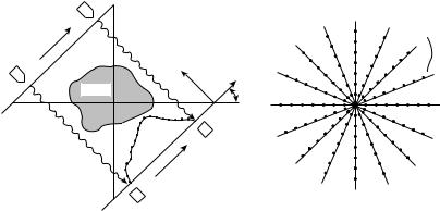
COMPUTED TOMOGRAPHY |
247 |
completion of even the first iteration, and they are very process intensive. Iterative techniques may be useful for selected situations where the data is limited or distorted, working with incomplete data sets, or with irregular data collection configurations. Known information on the object or object values may be incorporated into these techniques and reconstruction dependent corrections, such as for beam hardening, may be incorporated into the process. While not normally used for medical X-ray computed tomography, iterative techniques are commonly used in nuclear medicine SPECT and PET imaging. Variations may also be used in X-ray tomosynthesis that is a partial angle data acquisition technique used to generate planar images through an object, but without complete elimination of overlying structures (43).
Analytical Reconstruction Techniques
If one can analyze and solve a series of equations directly, it is an analytical technique. Radon in 1917 mathematically determined that a solution existed for determining the distribution of an object from a series of line integrals through it. Interesting though, is that Radon’s work was not utilized in the development of CT, but it was noted afterwards that it encompassed the analytic reconstruction methods. Applied developments of the principles used were often driven outside of X-ray imaging, including radio astronomy (8), electron microscopy (9), and nuclear medicine (10), and discovered methods were often not implemented due to computational requirements in the precomputer age.
Direct Fourier Reconstruction
The Fourier transform is a mathematical operation that converts the object distribution defined in spatial coordinates into an equivalent distribution of sinusoidal amplitude and phase values in spatial frequency. The one-dimensional (1D) Fourier transformation of a set of projection data at a particular angle u is given as
Z
Pðr; uÞ ¼ pðr; uÞe 2prrdr |
ð15Þ |
where r is the spatial position along the set of projection data and r is the corresponding spatial frequency variable.
|
|
y |
|
|
|
-ray |
tube |
|
|
|
|
|
|
|
|
|
|
X |
|
|
) |
|
|
|
|
ρ |
|
|
|
|
|
( |
|
|
|
|
|
θ |
|
|
|
|
|
P |
|
|
ρ |
|
Object |
|
|
|
|
|
|
|
θ |
x |
|
|
|
|
|
||
|
|
|
|
|
|
|
|
Detector |
|
|
|
(a) |
|
|
|
|
(b) |
The direct Fourier reconstruction technique, as well as the filtered backprojection method, are based on a mathematical relationship know as the central projection theorem or central slice theorem. This theorem states that the Fourier transform of a 1D projection through a 2D distribution is mathematically equivalent to the values along a radial line through the 2D distribution of the original distribution.
Taking the Fourier transform of one set of projection data measurements through an object at a particular angle provides data values along one spoke in the object’s 2D Fourier transform frequency space. Repeating this process for a number of angles defines the 2D Fourier transform of the object distribution in polar coordinates (Fig. 13). Taking the inverse Fourier transform of this data yields the reconstructed image of the object.
Direct Fourier technique is potentially the fastest method for image reconstruction, however, it generally does not achieve the image quality of the filtered backprojection method due to data interpolation difficulties. Typical computer methods and display systems are based on rectangular grids rather than polar distributions, and direct Fourier reconstructions generally require an interpolation of the data from polar coordinates to a Cartesian grid, usually performed in the frequency domain. Consequently, these methods are generally not used in commercial medical scanners.
Convolutions and Filters
The filtered-backprojection technique is the most commonly used CT reconstruction algorithm. Before discussing this method, a brief review of filtering and simple backprojection methods is in order.
A convolution is a mathematical operation in which one function is smeared by another function. A common example is a presentation of a blurry out-of-focus projection of a text slide. A small dot, such as a period, instead of being small, sharp, and dark gets blurry with smooth edges and less contrast or darkness. This blurry spot is effectively the point spread function of the image. All of the lines and characters in the original slide can be considered as being made up of many points. Replacing each of these points with the
Wy |
Spoke for the |
orientation of θ |
|
|
shown in (a) |
Wx |
Figure 13. According to the central-slice |
|
|
|
theorem, the 1D Fourier transform of the pro- |
|
jection values measured through an object in |
|
the spatial domain (a), correspond to the |
|
values of the 2D Fourier transform of the |
|
object along a diagonal line in the frequency |
|
domain. A series of transformed projection |
|
values yield the Fourier transform of the |
|
object, but in polar coordinates. |

248 COMPUTED TOMOGRAPHY
out-of-focus point results yields the overall blurry slide that is seen. The process of applying this blurry point to all points in the images is a convolution of the point spread function with the original object. Mathematically this is defined as
gðxÞ ¼ f ðxÞ hðxÞ |
ð16Þ |
||
|
1 |
|
|
gðxÞ ¼ Z |
f ðxÞhðx uÞdu |
ð17Þ |
|
|
1 |
|
|
for 1D, or for 2D |
|
|
|
gðx; yÞ ¼ f ðx; yÞ hðx; yÞ |
ð18Þ |
||
1 1 |
|
|
|
gðx; yÞ ¼ Z Z |
f ðx; yÞhðx u; y vÞdudv |
ð19Þ |
|
1 1
where the symbol is the convolution operator between two functional distributions. If the system is a digital system with a discrete number of samples, the corresponding equation is
|
1 |
|
gi ¼ kX fihiþk |
ð20Þ |
|
|
¼ 1 |
|
or in 2D |
|
|
1 |
1 |
|
gi; j ¼ kX l X fi; jhiþk; jþl |
ð21Þ |
|
¼ 1 ¼ 1 |
|
|
In the blurry slide example above, f may represent the original text (or image) distribution, h is the blur or point spread function, and g is the resultant blurred image.
Convolution operations can be used in image processing to smooth an image, as previously described, or to sharpen an image. Smoothing convolution filters are typically
square (averaging) or bell shaped, while sharpening convolution filters often have a positive central value with adjacent negative tails.
Convolution Theorem
Reference was made to Fourier transforms in Eq. 15 and their ability to transform spatial data into corresponding spatial frequency data. Filtering operations, such as smoothing and sharpening, can readily be performed on the data in the spatial frequency domain. According to the convolution theorem, convolution operations in the spatial domain correspond to a simple functional multiplication in the spatial frequency domain (Fig. 14). This states that
gðxÞ ¼ f ðxÞ hðxÞ |
ð22Þ |
is equivalent to |
|
GðkxÞ ¼ FðkxÞHðkxÞ |
ð23Þ |
where G(kx), F(kx), and H(kx) are the Fourier transformed functions of g(x), f(x), and h(x), where kx is the spatial frequency conjugate of x. The functional multiplication in Eq. 23 is simply the multiplication of values of F(kx) and G(kx) at all values of kx. The 2D convolution of Eq. 18 has its counterpart to Eq. 23 where G(kx,ky), F(kx,ky), and H(kx,ky) are the 2D Fourier transforms of g(x,y), f(x,y)and h(x,y). Note that the spatial frequency variables, kx and ky have units of 1/distance.
Since the convolution process is represented by a simple functional multiplication in the spatial frequency domain, the blurred image conceptually can be easily restored to the original object distribution. This can be accomplished by multiplying the Fourier transform of the blurred image, G(kx,ky), by the inverse of the blurring function, that is 1/H(kx,ky). The result is the original object frequency
Figure 14. The convolution theorem states that a convolution operation in the spatial domain is equivalent to the functional multiplication of the Fourier transform of the functions in the spatial frequency domain. The filtering of the projection data for CT reconstruction may be performed by the convolving the projection data with a sharpening filter in the spatial domain, or by taking the Fourier transform of the projection data, multiplying by a ramp shaped filter, and taking the inverse Fourier transform to yield the filtered projection data.
*
g (x) |
h′ (x) |
f (x) |
Fourier transform
x
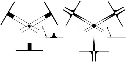
distribution, F(kx,ky). In practice this restoration is limited by the frequency limits of H(kx,ky) leading to division by zero, and by the excessive enhancement of noise along with the signal at frequencies with small H(kx,ky) values. This restoration process or deconvolution of the blurring function can likewise be performed as a convolution in the spatial domain.
Backprojection
Backprojection is the mathematical operation of mapping the 1D projection data back into a 2D grid. This is done intuitively by radiologists in interpreting X-ray films. If a high density object is visible in two or more radiographs taken at different angles, the radiologist mentally backprojects along the corresponding ray paths to determine the intersection of the rays within the patient and the location of the object.
Mathematically, this is done by taking each point on the 2D image grid and summing the corresponding projection value from each angular projection view. For that high density object the result is a line projected through the image from each view (Fig. 15a). This backprojection process yields a maximum density at the location of the object where the lines cross, but the lines form a star artifact emanating from the object. If an infinite number of views were used, the lines would merge and the density of the object would be smeared across the image with its amplitude decreasing with 1/r where r is the distance from the object. This simple backprojected image, fb,can be represented by the convolution of the true image, f, with the blurring function 1/r, or
fbðr; uÞ ¼ f ðr; uÞ ð1=rÞ |
ð24Þ |
With ideal data, this blurring function can be removed by a 2D deconvolution or filtering of the blurred image. The appropriate filter function can be determined by using the convolution theorem to transform Eq. 24 into it frequency domain equivalent, or
Fbðr; uÞ ¼ Fðr; uÞð1=rÞ |
ð25Þ |
COMPUTED TOMOGRAPHY |
249 |
where the function (1/r) is the Fourier transform of (1/r) in polar coordinates. Dividing both sides by (1/r) yields
Fðr; uÞ ¼ rFbðr; uÞ |
ð26Þ |
The corrected image, f, can be obtained by determining a simple backprojection, fb, taking its Fourier transform, filtering with the r function, and taking the inverse Fourier transform. Likewise this operation may be performed as a 2D convolution operation in the spatial domain. Equation 25 and 26 get more complicated when evaluated in rectangular coordinates rather than polar coordinates.
This approach of making a very blurred image through backprojection, and then attempting to sharpen the image tends to produce poor results with actual data. Filtering out this blurring function from the projection data prior to backprojecting, however, is quite effective and is the basis for the filtered backprojection reconstruction technique used in medical CT systems.
Filtered Backprojection Reconstruction Technique
According to the central slice theorem the Fourier transform of the 1D projection data is equivalent to the radial values of the 2D distribution Fourier transform of the distribution. Consequently, the filtering operation performed in Eq. 26 and illustrated in Fig. 14 can be performed on the projection data prior to backprojection. This is the conceptual basis for the filtered-backprojection reconstruction technique as illustrated in Fig. 15b (44,45).
As with other filtering operations, this correction can be implemented as a convolution in the spatial domain or as a functional multiplication in the frequency domain. Fourier filtered backprojection is performed by taking the measured projection data, Fourier transforming it into the frequency domain, multiplying by the ramp-shaped r filter, taking the inverse Fourier transform, and then backprojecting this filtered projection data onto the 2D grid.
If the filtering is performed in the spatial domain by convoluting the measured projection data with a spatial filter that is equivalent to the inverse Fourier transform of r, the process is often referred to as the convolution
|
|
|
|
|
|
|
Figure 15. (a) A simple backpro- |
|
|
|
|
|
|
|
|
|
|
|
|
|
|
|
|
|
|
|
|
|
|
|
|
|
|
|
|
|
|
|
|
|
|
|
|
|
|
|
jection from three views results in |
|
|
|
|
|
|
|
|
|
|
|
|
|
|
|
a highly blurred reconstruction. (b) |
|
|
|
|
|
|
|
Filter the projection data prior to |
|
|
|
|
|
|
|
backprojection corrects the data for |
Simple backprojection |
Filtered backprojection |
|
the backprojection induced blurring. |
||||

250 COMPUTED TOMOGRAPHY
filtered backprojection reconstruction method. The frequency filter, r, has the shape of a ramp and enhances high spatial frequencies of the projection data. The convolution function, or kernel, has the expected shape of a sharpening filter with a positive central value surrounded by negative tails that diminish in magnitude with distance from the center. Convolution and Fourier filtering techniques are mathematically equivalent and the general term filtered backprojection reconstruction technique may refer to either filtering approach.
Variations from this ideal ramp filter are normally used. Some of these may develop from applying the finite quantity of data and boundary assumptions to the mathematical derivation. Other variations, in particular frequency windowing, are applied on a more empirical basis. The high spatial frequency component of the projection data contains noise variations due to photon statistic along with diminishing amounts of signal data. The ramp filter greatly enhances these high frequency values, in particular the noise. Consequently, use of the ramp filter results in high resolution, but very noisy images. They are also more susceptible to image artifacts. If one wishes to see structures with only small differences in attenuation values, such as white versus gray brain matter, the noise must be reduced.
Medical CT scanners offer a variety of reconstruction algorithms or kernels from which to choose. In actuality they are not changing the reconstruction method, but the filter function used in the filtered backprojection technique. The ramp filter is modified by a windowing or apodizing filter that reduces the amplification of the higher frequency values. This has the same effect as smoothing the image. This smoothing is especially effective for CT imaging since the reconstruction process results in the noise frequency spectrum in the image following the reconstruction filter function, with most of the noise at the high spatial frequencies. In nuclear medicine they sometimes use the mathematical name for the windowing filter, such as cosine filter, Butterworth filter, or Hannings window. In X-ray CT the equipment manufacturers utilize different naming conventions for these filters kernels. Typically, they will have descriptive names, such as smooth, standard, sharp, bone, edge, or will have numerical values relating to its shape. The filter selection may also enable other features in the reconstruction process to minimize certain artifacts, such as motion in the body scans, or implement other needed data corrections.
The filtered backprojection reconstruction technique is the general method used in medical CT systems. This method is more tolerant of measured data imperfections than some of the other analytical techniques. This method provides relatively fast reconstructions and permits processing the data as projection views are obtained.
Cone Beam CT
Computed tomography scanning has progressed from a single row of detectors to the ability to use hundreds of rows of detectors for data acquisition. The CT reconstruction algorithms discussed above have generally considered all of the projection values being contained within a single plane through the patient. As one uses multiple rows of detectors, the projection data from the rows away from the
Figure 16. With a multislice detector or area detector, an axial (nonhelical) data acquisition results in rays outside of the center to pass through the patient at an angle rather than within a particular plane. This can cause artifacts in planar reconstructions. Specialized cone beam reconstruction algorithms may be used to help account for the angulated data.
center row pass through the patient at an angle. Objects within a view from one side may be outside to the view from the opposite view angle (Fig. 16). Generally, this angulation is ignored in the reconstruction, but data inconsistencies from the angulated data can cause artifacts in the image, especially around high density structures. Other algorithms are continuing to be developed that take into account the actual ray paths of the data (4). These algorithms are referred to as cone beam reconstruction methods.
With data acquired in an axial mode, with no table motion during data acquisition, large angulations cause significant degradation of the image quality, but may be useful in particular for high contrast structures such as bone or contrasted blood vessels. Considering the relationship between the object and the projection data, a simple rotation does not fully sample the Radon space needed for reconstruction. A helical data acquisition and certain other motion schemes do acquire a sufficient set of data for a potentially accurate cone beam reconstruction.
CT IMAGE QUALITY
A particular image will have limitations on the quality of the image and the types of structures that are visible. Two primary measures of image quality are the image resolution and noise (46). Resolution is the ability to see two separate small structures as two structures. It is somewhat different
that detection. A very small dense structure considerably smaller than the voxel size may change the average attenuation within the voxel sufficiently to detect that a foreign object is present, however, the system would not have sufficient resolution to distinguish multiple objects within the voxel.
Resolution may be measured by using a test pattern of holes that are spaced with the center-to-center distance between holes being equal to twice the hole diameter. Alternatively, the pattern may be a series of lines or bars, or a pie shaped wedge of bars that get smaller toward the apex of the pattern. The resolution is usually stated as the hole or bar size of the smallest pattern clearly visible, or as a spatial frequency value in line pairs per millimeter (lp mm 1). The resolution may be more precisely described by determining the modulation transfer function or MTF. This function indicates the level of signal loss for each of the spatial frequencies. The MTF is the normalized Fourier transform of the point spread function, and can be calculated by analyzing the image of a small dense object, or from measurements across a sharp boundary (47).
Geometric Blurring
A number of factors can affect the resolution in an image, some inherent in the design and construction of the system, and others selectable by the user. Limits on resolution for a system are generally determined by the detector width and the focal spot size of the X-ray source. Since the patient is approximately midway between the source and detector, there is necessarily some magnification of the object structures onto the detector. As a result of this magnification a sharp edge in the object will produce a blurry edge in the image due to the size of the X-ray source. This blurry area where only part of the X-ray source illuminates the detector is called the penumbra from the Latin for partial shadow, and the effect is referred to as geometric blurring. This sharpness can be improved by reducing the magnification, which is done by having the X-ray source farther from the patient and the detector as close to the patient as possible. It can also be improved by use of a smaller X-ray focal spot. Most X-ray tubes utilize a dual focal spot, which means they have two focal spot sizes from which to choose. Most scanning is done with the large focal spot. This allows operation at higher tube currents or mA, thereby allowing shorter scan times and less image noise. This is especially true for large field-of-view objects where this geometric blurring is not the limiting factor for resolution. Scanners will typically select the smallest focal spot that can be used with the mA and time parameters selected.
Ray Spacing
The detector size may also affect the resolution. For a rotate–rotate scan system, the in-plane detector-to- detector spacing defines the ray spacing within a view. Note that this ray spacing is variable due to the fan shape of the beam, but consider it at the center of rotation, which is normally the center of the patient. The detector size has decreased with the evolution of the scanners, resulting in the need for an increase in the number of detector channels and the amount of data gathered and processed. Since the physical detector spacing cannot readily be changed for a
COMPUTED TOMOGRAPHY |
251 |
given detector, a couple of alternative approaches have been used to change the effective ray spacing. An approach that has been used in the past maintains a fixed source– detector distance, but moves the X-ray tube closer to the patient, and the detector farther away when scanning smaller objects, such as the head. This increases the magnification and reduces the ray spacing, but puts more of a resolution burden on the size of the focal spot. No commercial systems still use this approach.
A common approach in rotate–rotate scanners is to improve sampling by using quarter–quarter offset detector shift. First generation translate–rotate scanners acquired data only > 1808 of rotation since the view at 08 is of the same data as the 1808 view. If the ray spacing is not symmetric about the center of rotation, but the middle ray being displaced one-quarter of a detector width above the center of rotation, then the opposite view would have the ray one-quarter of a detector width below the center of rotation and the rays would be interleaved. It is not as obvious on a rotate–rotate scanner, but the same type of interleaving can be utilized. A rotate–rotate scanner only needs 1808 plus a fan angle to sufficient set of data for a reconstruction. Certain fast scan modes will utilize this partial rotation data set, but typically the full 3608 data set is used. In high resolution reconstructions, the full 3608 data set should be used.
Pixel Size
The CT image is a finite array of values. Parameters selectable setting up the image reconstruction include the reconstructed field of view (FOV), and the image matrix size. Images are routinely reconstructed with a 512 512 matrix. The large FOV that would be used for a large body section is 50 cm. Therefore the generated pixels will be squares with sides of 50 cm/512 or 1 mm. In this case, the image would not be effective at resolving or differentiating objects smaller than this pixel size. Medical CT systems have the capability to provide better resolution than can be displayed with 1 mm pixels. To reduce the pixel size the image matrix size must be increased, or the reconstructed FOV reduced. The reduction in FOV is standard for imaging smaller body sections, such as the head where a 25 cm FOV may be used. This yields a 0.5 mm pixel size. If higher resolutions are desired, such as to evaluate the bones of the inner ear, then a sharp reconstruction filter is needed along with an even smaller pixel size in order to maximize the system resolution. Unfortunately these parameter changes also increase the image noise.
Image Magnification and Targeted Reconstructions
A number of display tools are available when an image is displayed. These include such useful features as the window level and width adjustments. One tool is image magnification where a portion of the original image can be magnified to fill the display or a digital magnifying glass can be moved around the screen. This function uses the data from the image and interpolates additional pixels to yield smaller pixel spacing. Since the source data is the original image, the magnified image does not contain any

252 COMPUTED TOMOGRAPHY
additional information, but the viewer may find it easier to see and interpret the image.
This image magnification is in contrast to a targeted reconstruction that goes back to the measured projection data and performs a reconstruction with new parameters such as reconstruction filter and pixel size. Consequently, a targeted reconstruction may yield information that was not present in the original image. In the case of helical scans and multislice detectors, the z-axis location of the reconstructed slices and the slice thickness, down to the acquisition detector row thickness, may also be specified.
z-Axis Resolution
The z-axis resolution is the resolution in the direction of the table motion or perpendicular to the axial image plane. The acquisition slice thickness and slice spacing dominate this resolution. The slice spacing limitation on z-axis resolution follows the same arguments as the pixel size does for the x–y resolution. The slice thickness is determined by the focal spot size and either the collimated beam thickness or the z-axis height of the detector. For multislice detectors, the detector rows may be utilized individually, or ganged together to yield a thicker slice, or both with the averaging of detector rows performed in the software. A major advantage to MDCT and cone beam CT is the ability to rapidly acquire many thin slices through the patient. This often results in isotropic resolution where the resolution in the z axis is equivalent to the in-plane resolution. These thinner slices and isotropic resolution improves the contrast of small high contrast structures, such as the blood vessels of the lung. The thin closely spaced slices greatly improve the quality of images that contain the z dimension, such as sagittal and coronal images, or 3D surface reformations.
Image Noise
Another significant limitation to image quality is image noise or graininess. Noise is caused by variations in the measured signal. These may be due to systemic causes, such as electronic noise, however, a well-designed system will not be limited by these sources. The primary source of noise in medical CT systems is due to quantum mottle or photon statistics. Due to the random nature of photon emission and absorption, repeated identical measurements will vary with a percent standard deviation proportional to one over the square root of the number of photons detected, that is
|
¼ |
p |
|
|
|
ð27Þ |
|
s |
|
N |
|
|
|
||
%s |
100% |
|
p |
28 |
|||
¼ |
|
|
|
|
|
N |
ð Þ |
|
|
|
N |
||||
%s ¼ |
|
|
|
|
|
|
ð29Þ |
100% p1 |
|||||||
N
where s is the standard deviation and N is the number of photons detected. The number of photons detected is determined by the output of the radiation source, the attenuation in the patient, and the efficiency of the
detector in absorbing the radiation and converting it into a measurable signal. The source output is directly proportional to the selected tube current or mA, and the scan time per rotation and to the kVp to some power 3. The beam is diminished by attenuation, hence noise is more prevalent scanning a large body section. Higher kVp settings are more penetrating and allow a larger fraction of the photons through the patient, but may also reduce the contrast of some structures.
Another factor is the size of the detector, in particular the detector height or the slice thickness. Thinner slices result in fewer X rays for a given technique. Helical scanning interpolates data from adjacent rotations, thereby increasing the effective slice thickness and reducing the noise to some degree. The image resolution and pixel size also can have an effect. One can consider the image noise to be related to the number of photons detected per voxel element. Reducing the voxel or resolution element size increases the noise.
Noise can be expressed as the standard deviation in the image of a uniform object. A more complete method of characterizing noise is to determine the noise power spectrum. The noise power spectrum defines the noise content in the image versus spatial frequency. The measure transmission data ideally contains white noise, that is, having a noise power spectrum at all frequencies. As with other imaging systems this ideal spectrum is modified by the modulation transfer function (MTF) or ability of the system to transfer signal (and noise) of various frequencies in the object to the image. The resolution limitations due to detector size and sampling reduces or eliminates some high frequency signal components. In CT, there is the additional step of the image reconstruction which modifies the noise power spectrum. The projection data is filtered with a ramp or a windowed ramp filter, reducing the low frequency content and enhancing the medium and high frequency content. For signal data where there is a correspondence in the data from various angles, the low frequency component is restored and a typical MTF response is generated. The noise content, however, is random and does not have a direct correspondence between angles. Consequently, the noise power spectrum will mimic the shape of the filtering function, enhancing noise at the higher spatial frequencies. Smoothing or the use of a windowed filter is especially effective in CT since there is a high level of noise relative to signal at these frequencies (48).
Object Contrast
Contrast is the difference in the measured value of a structure from its surroundings. The ability to distinguish structures that have attenuation differences of a fraction of a percent is one of the key imaging benefits of CT. The contrast between structures in CT is the fractional difference in attenuation coefficient, or more commonly the difference in attenuation coefficient relative to the attenuation coefficient of water. This is given by
% Contrast ¼ |
jm mbackgroundj |
100% |
ð30Þ |
mwater |

When CT values have an offset of 1000 in order to normalize water to a value of zero, the comparable equation using the CT values is
% Contrast ¼ jCT CTbackgroundj 100%
1000
For example, if brain gray matter has a CT number of 40 and white matter 30, then the fractional contrast is 10/1000 or 1%.
One of the factors that often limits contrast is the partial volume effect. Voxels or resolution volumes that correspond to a particular pixel may contain a mixture of tissues or structures. The resultant CT number is generally a volume average of the contents of the voxel. Reducing the voxel size with thinner slice thickness or higher image resolution may reduce this volume averaging. For example, a 1 mm piece of bone that is twice as attenuating as water (CT number of þ 1000) is surrounded by water (CT number of 0). If scanned with a 10 mm slice thickness, the bone would occupy 10% of the voxel volume and the resultant image would show a CT number for this volume of 100. Reducing the slice thickness to 2 mm would increase the CT number to 500. This is not an error or image artifact, but a limitation in the image quality and content. If structures are positioned in the voxel such that part of the ray goes through one material, and other portions of the ray go through other material, this may cause a measurement error and a partial volume artifact.
The linear attenuation coefficient values are a function of the density of the material and effective atomic number of the material, as well as the effective energy of the X-ray beam. Sometimes there is insufficient contrast between a structure of interest and its surroundings, or certain structures are to be highlighted. This may be done through the use of contrast agents or contrast media. This is a material that will change the X-ray absorption properties and the visibility of the structure. In X-ray studies the primary contrast agent used is iodine, which may be given orally to highlight the intestinal track, or injected to make blood vessels or highly vascular tissue visible. The iodine does not actually change the density of the blood significantly, but its higher atomic number of 56 versus 7 or 8 for tissue and water, and its k shell electron binding energy of 34 keV make it much more effective at stopping the X rays. Using contrast media the radiologist may determine the vascularity of a mass to help determine the type of tumor, or contrast agents can be used to enhance the blood vessels to evaluate blockages or aneurysms in CT angiography procedures.
Low Contrast Detectability
The ability to see small differences in contrast is a key feature of CT. What limits this ability, however, is noise. When the noise variations are of the same magnitude as the contrast between the structures of interest, the structure will not be visible. This is especially true for small objects, in that the human vision will effectively average the signal over an area and one may be able to distinguish larger low contrast objects. The limit to low contrast detectability is noise and resolution has relatively little impact
COMPUTED TOMOGRAPHY |
253 |
(Fig. 17c–e). Conversely, high contrast resolution is not greatly affected by noise since the structures contrast is much larger than the noise.
ARTIFACTS
The ideal imaging system reproduces a faithful image of the object. Limitations in resolution, noise, and low contrast detectability are not errors, but are definable limitations of particular imaging systems. Errors do occur, however, and structures or patterns may appear in the image that do not correspond to the patient or object being scanned. These false structures in an image are referred to as artifacts (49). Artifacts often are readily identifiable because of their characteristics, such as a bright line extending through and beyond the boundaries of the patient. These artifacts may cause problems by obscuring parts of the image. Less common, but of significant concern, are artifacts that can appear similar to pathologies.
Artifacts occur in all imaging systems, but the reconstruction process of CT enhances the opportunity for producing artifacts. Mathematically a perfect reconstruction of the object should be obtainable. This can be done with an infinite amount of perfect data, however this is not available in a practical system. In general, image artifacts are caused by an insufficient amount of data, or insufficient quality of data.
Insufficient Data Quantity
Modern CT scanners acquire millions of transmission measurements and insufficient data quantity is not a limiting factor for routine studies, but still may pose challenges in studies attempting to reduce the data acquisition time or those pushing the image resolution. Nyquist sampling theorem was mentioned as a requirement for sampling an object in order to capture the high spatial frequencies. When the object contains higher frequencies than the sampling rate can characterize, the high frequencies reappear in the data and take on the alias of a lower spatial frequency. The resulting error is referred to as aliasing. It can take on the appearance of ripples in the reconstructed object parallel to a sharp edge.
Aliasing may occur due to insufficient sampling of rays within a view, or may be due to an insufficient number of views. Ray aliasing may appear as oscillations or ripples parallel to high contrast. View aliasing typically appears a considerable distance from a high contrast object, and appear as a radial pattern of light and dark bands emanating from the high contrast object.
The occurrence of aliasing is greatly reduced by the data smoothing effect that occurs due to the finite size of the X-ray detector. The transmission data is not measuring a series of infinitely thin rays, but columns through the patient. The variations in intensity between the various paths within a single ray or detector measurement get averaged out and lost, and are not available to cause aliasing.
A related artifact is the Gibb’s phenomena. The range of the frequency domain is limited by the sample spacing. Using the full ramp function results in an abrupt cutoff of the filter function or transfer function at this limit, or the
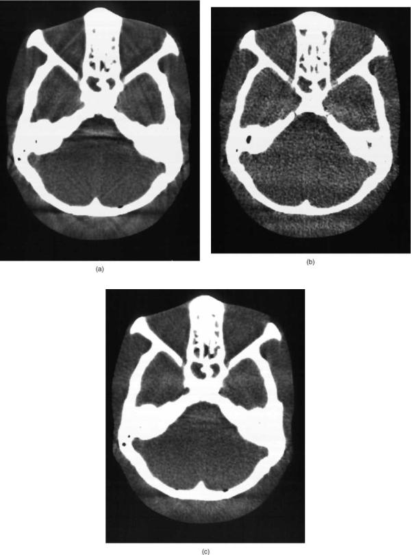
254 COMPUTED TOMOGRAPHY
Figure 17. (a) A 5 mm thick CT slice through the posterior fossa can cause beam hardening and partial volume artifacts as seen in this acrylic phantom containing a skull. (b) Use of a thinner 1 mm slice thickness reduces the partial volume artifact from the angled bony structures, but increases the image noise orgraininess.(c) Adding five1 mm slicestogether (or the fivesets ofprojectiondataafter the logarithmic scaling) results in reduced artifact, but comparable image noise as the 5 mm slice.
filter may be designed with a sharp cutoff. This sharp edge in the frequency domain causes an overshoot and ringing artifact along edges in the image. This can be reduced by windowing the filter function with a function that smoothly goes to zero without an abrupt change.
Inconsistent Data
The CT reconstruction process is based on obtaining a consistent set of transmission views of the patient from various angles. The reconstruction algorithms effectively correct for errors caused in the backprojection from one view with corrections in other views. If the object or data is not consistent, then improper corrections are applied resulting in artifacts. There are several factors that can cause data inconsistencies and result in artifacts.
Motion
One of the most obvious inconsistencies is patient motion, whether squirming, coughing, fluid level movements in the stomach, breathing, or even the beating of the heart. Here the views from different angles are not of the same crosssectional object. Motion artifacts are less of a problem in head imaging since with a cooperative patient the head can remain motionless for a considerable period of time. Body imaging can be more problematic causing image artifacts in addition to the motion blurring in the image.
The artifact is most pronounced when there is an abrupt change in the data from one view to the next usually resulting in streaks across the image. For a 3608 data acquisition this abrupt change in the continuity of the data is likely to occur between the first and last view of the rotation. There are several ways to minimize this. One can overscan, collecting > 3608 of data, and perform a weighted average of the data in the overlap region. Partial angle scanning, scanning 1808 plus a fan angle, reduces this interface effect and reduces scan time, but also reduces image quality. The data may use a variable weighting of the data at the first–last view interface region reducing artifacts, but may increase noise some and result in the noise structure having a directional pattern toward this start–stop angle. This may be seen on some body scans but typically would not be used or present in head scans.
One of the obvious improvements in reducing motion artifacts is the use of shorter scan times. In early scanners it took tens of seconds to minutes to scan a single image, much less a volume through the patient. With MDCT and cone beam scanning, one can scan the entire chest within a breathhold. If one is looking at cardiac structures, however, the motion is rapid and less controllable. At times the motion may cause the image of a structure at one point in time overlaid on the image of the structure at a different point in time. This can cause artifacts that may mimic a pathology and special care is needed regarding this type of artifact. One example is imaging of the aorta as it changes diameter with the beating of the heart may create the image of a double vessel wall, which could look similar to a dissecting aneurysm (50). The electron beam CT systems were developed to provide very fast, freezeaction scans, and the use of cardiac gating to selectively
COMPUTED TOMOGRAPHY |
255 |
collect data through the heart during defined portions of the cardiac cycle also reduce motion artifacts and blurring.
Partial Volume Artifact
Equation 12 in the discussion of the attenuation of X rays shows that a beam passing through a series of objects yields a relative transmission value that is the exponential of a sum of ms values. Taking the logarithm of this value yields the projection data that is the sum or integral of attenuation values along a line through the object. The X-ray beam that strikes a single detector is not a single infinitely slender beam, but a beam of some finite cross-sectional area. If part of the beam passes through one structure, and the other part of the beam passes through another structure, then the resulting transmission values corresponds to a sum of two or more exponentials, rather than an exponential of a sum. Taking the logarithm of this does not yield the same results. This can be seen by the example of a beam passing through a series of alternating dense and radiolucent layers will eventually get infinitesimally small. The same beam, however, having half of the beam transverse the dense material, and half the beam travel through the radiolucent material will always transmit at least 50% of the beam through the radiolucent path. This difference in attenuating material for different parts of a measured ray is commonly present along long linear boundaries. If the difference in density of the two materials is small, then there is little effect, but if there is a large difference in attenuation between the materials, such as for bone or a metal structure, then these inconsistencies result in streaks emanating as an extension of the edge (Fig. 17a).
This partial volume artifact is also produced by structures that penetrate only part way through the slice thickness, and may cause streaks between such partially penetrating structures. Partial volume streak artifacts may be reduced by reducing the slice thickness, which reduces the cross-sectional area of the measured ray. This can be especially useful in high resolution imaging of structures with bony prominences (Fig. 17b and c), or in the presence of dense metal structures (Fig. 18). The routine use of thinner detectors in MSCT systems, even when the detectors are averaged together as long as it is after the logarithmic scaling, reduces this artifact.
A related artifact is the windmill artifact due to insufficient sampling in the z axis in helical scanning. This presents as fan shaped lines emanating from edges. Increased sampling or lower pitch can reduce this artifact. Alternatively, view spacing in the axial direction may be reduced by using a flying focal spot approach that rapidly moves the position of the X-ray source in the X-ray tube. This uses an oscillating magnetic field to alter the path of the electrons and the location on the X-ray tube target where the electrons strike.
Beam Hardening Artifact
The attenuation parameters used in Eqs. 10–14 assumed a monoenergetic X-ray source yielding consistent values of m for a given material. However, X-ray sources produce
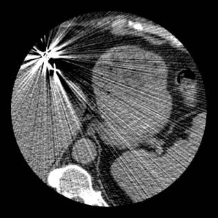
256 COMPUTED TOMOGRAPHY
Figure 18. Dense metal structures in the body can produce pronounced streaking artifacts. Partial volume edge artifacts, beam hardening, scatter, and motion can all contribute to inconsistencies in the data causing the artifacts.
radiation with a range of photon energies up to the maximum energy of the electrons striking the X-ray tube target. This maximum photon energy corresponds to the kV or kVp voltage applied to the tube. The lower energy or soft photons are attenuated to a greater degree than the more penetrating high energy photons. Consequently, the effective energy of a beam passing through a thick object section is higher than that of a beam going through less material. This preferential transmission of the higher energy photons and the resulting increase in effective energy of the X-ray beam is referred to as beam hardening.
The linear attenuation coefficient is a function of the beam energy and changes in beam energy cause variations in the CT number for a material. Likewise, if rays passing through an object from different angles have different effective energies, then the inconsistencies can also cause artifacts. X-rays that pass through the center of a cylindrical object will have higher effective energy than those traversing through the edges. This additional attenuation and beam hardening of the central rays result in lower CT number values in the center, corresponding to the higher energy beam. This appearance of lower CT numbers in the center of an object is referred to as a cupping artifact.
Another type of beam hardening artifact occurs between two dense structures. The rays passing through two dense structures have increased beam hardening, and tissues between these structures will appear to have a lower CT value. This appears as a dark band between the structures, and may be present along with partial volume artifacts appearing as fine streaking from edges. This is often seen in head scans as dark bands between the petrous ridges (Fig. 17a).
The effect of beam hardening can be reduced by several techniques. The original EMI scanner used a constantlength water bath that resulted in a relatively uniform degree of attenuation from the center to the periphery. The addition of X-ray beam filtration reduces the soft X rays and reduces the degree of beam hardening (51). Bow-tie shaped compensating X-ray filters are often used and attenuate the beam more toward the periphery. Normalizing the data with a cylindrical object of similar size and material also reduces beam hardening as well as minimizing detector variation errors.
Beam hardening is also compensated for in the processing software. If the material being scanned is known, the measured transmission value can be empirically corrected. Difficulty occurs when the object consists of multiple materials with different effective atomic numbers, such as the presence of bone or metal in the tissue. Iterative beam hardening corrections can be used, where the initial reconstruction identifies the dense structures, and the rays through these structures are corrected for a second reconstruction. Dual energy scanning techniques can also eliminate beam-hardening effects.
Scatter Radiation
Detected scatter radiation produces a false detected signal that does not correspond to the transmitted intensity along the measured ray. Scatter is a factor in all radiographic measurements. The amount of scatter radiation detected in CT is much lower than encountered with large area radiographs due to the thin fan beam normally used in CT. Most of the scatter is directed outside of the fan beam and is not detected. The sensitivity of computed tomography, and the need for consistent data makes even the low level of scatter detected a potential problem. The amount of scatter and this problem becomes more challenging as the collimated beam width gets larger with MDCT and cone beam systems.
The scatter contribution across the detector array tends to be a slowly varying additive signal. The effect on the measured data is most significant for highly attenuated rays where the scatter signal is relatively large compared to the primary signal. The additional scattered photons detected make the materials along the measured ray appear less attenuating, in a manner similar to beam hardening. Because of the similarity of these effects, scattering artifacts are similar to and are often associated with beam hardening. Likewise, the basic beam hardening correction performed provides some degree of compensation for scatter. Using thin beams and large distances between the patient and detector can minimize scatter. The use of directional dependent detectors such as the xenon gas ionization detectors with their focused tungsten plates can also reduce the detection of scatter. As detectors get larger with cone beam CT applications, scatter is significant and antiscatter radiographic grids can be used to reduce the detected scatter. Since scatter varies slowly with distance, special reference detectors outside of the primary radiation beam can be used to measure the level of the scatter signal for more effective correction.

Cone Beam or Divergence Errors
The X-ray fan beam does not only diverge or fan out in the x–y plane, perpendicular to the rotational axis, but also a slight divergence in the z direction, across the detector row (Fig. 16). A high density structure toward the edges of the patient may be in the x-ray beam from one angle, but be missing the beam from the opposite angle. This inconsistency causes an artifact that may include diffuse streaking or smearing of the density from the edges of the object. This may also occur in a helical data acquisition that interpolates the data to produce a data set corresponding to a given slice. Alternative variations in the reconstruction process that utilize a cone beam reconstruction approach or backproject along the actual ray paths reduce this effect.
Note that a single axial rotation around the patient with a widely diverging beam with an area detector does not contain a complete set of projection data sufficient to perform a reconstruction. Mathematically, it does not fully sample the Radon space. Reconstructions can be performed with various means to estimate the missing data, with the difficulty increasing as the divergence perpendicular to the plane of rotation gets larger.
Other Systemic Errors
There are a lot of things that can happen to the signal between the X-ray source and the image. Computed tomography scanners are complex electromechanical devices that are sensitive to relatively small variations in the measurements. A number of factors can cause accuracy or inconsistency errors and result in artifacts, and considerable effort is taken by the manufacturers to minimize these problems and artifacts. These inconsistencies may be in the measured signal or may be the result of poor characterization of the spatial position or the measured ray path. Geometric errors can result in wobble of the center of rotation due to the mechanical limitations of the large turret bearing holding the rotating mechanism, or may be due to small changes in the focal spot position as the X-ray tube gets hot, or variations in the spacing or position of the individual detector elements.
Signal variations occur due to fluctuations in the X-ray tube output, and differences in response characteristics among the individual detector elements. Periodic calibration of the detectors is required and radiation sensors are used to monitor variations in the X-ray tube output. Typically the reference detectors are at the ends of the linear detector array. A large patient, or body part outside of the normal scan field of view can block the reference detector, causing an inaccurate normalization of the measurements. Alternatively, an X-ray sensor may be placed adjacent to the X-ray tube where the measurement cannot be blocked. Vibrations in components can also affect the readings, as well as a number of other factors.
Detector calibration and characterization is particularly important with rotate-rotate data acquisition systems. The ray paths for a single detector all are tangential to a circle around the center of rotation. A relatively small consistent error in a detector can accumulate to form a ring artifact in
COMPUTED TOMOGRAPHY |
257 |
Figure 19. Ring artifacts centered on the scanner’s center of rotation can be caused by the miscalibration or error in a single radiation detector on a rotate–rotate data acquisition CT scanner.
the image (Fig. 19). The commercial X-ray CT systems are designed to be as stable and consistent as practical, however characterization of the various components and software correction of the measured transmission data is an important step in clinical CT imaging.
BIBLIOGRAPHY
1.Hounsfield GN. Computed medical imaging. J Computer Assist Tomogr 1980;5:665–674.
2.Brooks R, DiChiro G. Principles of computer assisted tomography (CAT) in radiographic and radioisotopic imaging. Phys Med Biol 1976;21:689–732.
3.Radon J. Uber die bestimmung von funktionen durch ihre Integralwerte langs gewisser Mannigfaltigkeiten. Ber Verhandlung 1917;69:262–277.
4.Feldkamp LA, Davis LL, Kress JW. Practical cone-beam algorithm. J Opt Soc Am 1984;1:612–619.
5.Herman GT. Image Reconstruction from Projections: Implementation and Applications. New York: Springer-Verlag; 1979.
6.Parker JA. Image Reconstruction in Radiology. Boca Raton: CRC Press; 1990.
7.Gordon R, Bender R, Herman GT. Algebraic reconstructioni techniques (ART) for three-dimensional electron microscopy and x-ray photography. J Theor Biol 1970;29:471–481.