Biosignal and Biomedical Image Processing MATLAB based Applications - John L. Semmlow

step response: a 15th order Parks–McClellan; a 15th-order rectangular window; a 30th-order rectangular window; and a 15th-order least squares firls. Use a bandwidth of 0.15 fs/2.

5.Repeat Problem 4 for four different IIR 12th-order lowpass filters: Butterworth, Chebyshev Type I, Chebyshev Type II, and an elliptic. Use a passband ripple of 0.5 db and a stopband ripple of 80 db where appropriate. Use the same bandwidth as in Problem 4.

6.Load the data file ensemble_data used in Problem 1 in Chapter 2. Calculate the ensemble average of the ensemble data, then filter the average with a 12th-order Butterworth filter. Select a cutoff frequency that removes most of the noise, but does not unduly distort the response dynamics. Implement the Butterworth filter using filter and plot the data before and after filtering. Implement the same filter using filtfilt and plot the resultant filter data. How do the two implementations of the Butterworth compare? Display the cutoff frequency on the one of the plots containing the filtered data.

7.Determine the spectrum of the Butterworth filter used in the above problem. Then use the three-stage design process to design and equivalent Parks–McClel- lan FIR filter. Plot the spectrum to confirm that they are similar and apply to the data of Problem 4 comparing the output of the FIR filter with the IIR Butterworth filter in Problem 4. Display the order of both filters on their respective data plots.

8.Differentiate the ensemble average data of Problems 6 and 7 using the twopoint central difference operator with a skip factor of 10. Construct a differentiator using a 16th-order least square linear phase firls FIR with a constant upward slope until some frequency fc, then rapid attenuation to zero. Adjust fc to minimize noise and still maintain derivative peaks. Plots should show data and derivative for each method, scaled for reasonable viewing. Also plot the filter’s spectral characteristic for the best value of fc.

9.Use the first stage IIR design routines, buttord, cheby1ord, cheby2ord,

and elliptord to find the filter order required for a lowpass filter that attenuates 40 db/octave. (An octave is a doubling in frequency: a slope of 6 db/octave = a slope of 20 db/decade). Assume a cutoff frequency of 200 Hz and a sampling frequency of 2 kHz.

10.Use sig_noise to construct a 512-point array consisting of two widely separated sinusoids: 150 and 350 Hz, both with SNR of -14 db. Use a 16-order Yule–Walker filter to generate a double bandpass filter with peaks at the two sinusoidal frequencies. Plot the filter’s frequency response as well as the FFT spectrum before and after filtering.

Copyright 2004 by Marcel Dekker, Inc. All Rights Reserved.

5

Spectral Analysis: Modern Techniques

PARAMETRIC MODEL-BASED METHODS

The techniques for determining the power spectra described in Chapter 3 are all based on the Fourier transform and are referred to as classical methods. These methods are the most robust of the spectral estimators. They require little in the way of assumptions regarding the origin or nature of the data, although some knowledge of the data could be useful for window selection and averaging strategies. In these classical approaches, the waveform outside the data window is implicitly assumed to be zero. Since this is rarely true, such an assumption can lead to distortion in the estimate (Marple, 1987). In addition, there are distortions due to the various data windows (including the rectangular window) as described in Chapter 3.

Modern approaches to spectral analysis are designed to overcome some of the distortions produced by the classical approach and are particularly effective if the data segments are short. Modern techniques fall into two broad classes: parametric, model-based* or eigen decomposition, and nonparametric. These techniques attempt to overcome the limitations of traditional methods by taking advantage of something that is known, or can be assumed, about the source signal. For example, if something is known about the process that gener-

*In some semantic contexts, all spectral analysis approaches can be considered model-based. For example, classic Fourier transform spectral analysis could be viewed as using a model consisting of harmonically related sinusoids. Here the term parametric is used to avoid possible confusion.

Copyright 2004 by Marcel Dekker, Inc. All Rights Reserved.

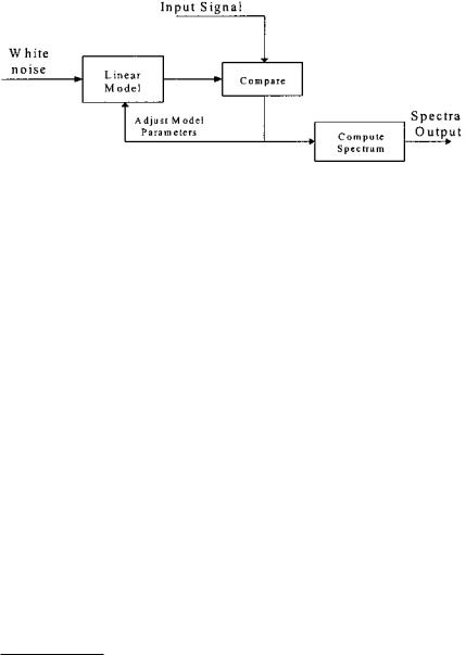
FIGURE 5.1 Schematic representation of model-based methods of spectral estimation.

ated the waveform of interest, then model-based, or parametric, methods can make assumptions about the waveform outside the data window. This eliminates the need for windowing and can improve spectral resolution and fidelity, particularly when the waveform contains a large amount of noise. Any improvement in resolution and fidelity will depend strongly on the appropriateness of the model selected (Marple, 1987). Accordingly, modern approaches, particularly parametric spectral methods, require somewhat more judgement in their application than classical methods. Moreover, these methods provide only magnitude information in the form of the power spectrum.

Parametric methods make use of a linear process, commonly referred to as a model* to estimate the power spectrum. The basic strategy of this approach is shown in Figure 5.1. The linear process or model is assumed to be driven by white noise. (Recall that white noise contains equal energy at all frequencies; its power spectrum is a constant over all frequencies.) The output of this model is compared with the input waveform and the model parameters adjusted for the best match between model output and the waveform of interest. When the best match is obtained, the model’s frequency characteristics provide the best estimate of the waveform’s spectrum, given the constraints of the model. This is because the input to the model is spectrally flat so that the spectrum at the output is a direct reflection of the model’s magnitude transfer function which, in turn, reflects the input spectrum. This method may seem roundabout, but it permits well-defined constraints, such as model type and order, to be placed on the type of spectrum that can be found.

*To clarify the terminology, a linear process is referred to as a model in parametric spectral analysis, just as it is termed a filter when it is used to shape a signal’s spectral characteristics. Despite the different terms, linear models, filters, or processes are all described by the basic equations given at the beginning of Chapter 4.

Copyright 2004 by Marcel Dekker, Inc. All Rights Reserved.

A number of different model types are used in this approach, differentiated by the nature of their transfer functions. Three models types are the most popular: autoregressive (AR), moving average (MA), and autoregressive moving average (ARMA). Selection of the most appropriate model selection requires some knowledge of the probable shape of the spectrum. The AR model is particularly useful for estimating spectra that have sharp peaks but no deep valleys. The AR model has a transfer function with only a constant in the numerator and a polynomial in the denominator; hence, this model is sometimes referred to as an all-pole model. This gives rise to a time domain equation similar to Eq.

(6) in Chapter 4, but with only a single numerator coefficient, b(0), which is assumed to be 1:

k=1

where u(n) is the input or noise function and p is the model order. Note that in Eq. (1), the output is obtained by convolving the model weight function, a(k), with past versions of the output (i.e., y(n-k)). This is similar to an IIR filter with a constant numerator.

The moving average model is useful for evaluating spectra with the valleys, but no sharp peaks. The transfer function for this model has only a numerator polynomial and is sometimes referred to as an all-zero model. The equation for an MA model is the same as for an FIR filter, and is also given by Eq. (6) in Chapter 4 with the single denominator coefficient a(0) set to 1:

k=1

where again x(n) is the input function and q is the model order*.

If the spectrum is likely to contain bold sharp peaks and the valleys, then a model that combines both the AR and MA characteristics can be used. As might be expected, the transfer function of an ARMA model contains both numerator and denominator polynomials, so it is sometimes referred to as a pole– zero model. The ARMA model equation is the same as Chapter 4’s Eq. (6) which describes a general linear process:

In addition to selecting the type of model to be used, it is also necessary to select the model order, p and/or q. Some knowledge of the process generating

*Note p and q are commonly used symbols for the order of AR and MA models, respectively.

Copyright 2004 by Marcel Dekker, Inc. All Rights Reserved.

the data would be helpful in this task. A few schemes have been developed to assist in selecting model order and are described briefly below. The general approach is based around the concept that model order should be sufficient to allow the model spectrum to fit the signal spectrum, but not so large that it begins fitting the noise as well. In many practical situations, model order is derived on a trial-and-error basis. The implications of model order are discussed below.

While many techniques exist for evaluating the parameters of an AR model, algorithms for MA and ARMA are less plentiful. In general, these algorithms involve significant computation and are not guaranteed to converge, or may converge to the wrong solution. Most ARMA methods estimate the AR and MA parameters separately, rather than jointly, as required for optimal solution. The MA approach cannot model narrowband spectra well: it is not a highresolution spectral estimator. This shortcoming limits its usefulness in power spectral estimation of biosignals. Since only the AR model is implemented in the MATLAB Signal Processing Toolbox, the rest of this description of modelbased power spectral analysis will be restricted to autoregressive spectral estimation. For a more comprehensive implementation of these and other models, the MATLAB Signal Identification Toolbox includes both MA and ARMA models along with a number of other algorithms for AR model estimation, in addition to other more advanced model-based approaches.

AR spectral estimation techniques can be divided into two categories: algorithms that process block data and algorithms that process data sequentially. The former are appropriate when the entire waveform is available in memory, while the latter are effective when incoming data must be evaluated rapidly for real-time considerations. Here we will consider only block-processing algorithms as they find the largest application in biomedical engineering and are the only algorithms implemented in the MATLAB Signal Processing Toolbox.

As with the concept of power spectral density introduced in the last chapter, the AR spectral approach is usually defined with regard to estimation based on the autocorrelation sequence. Nevertheless, better results are obtained, particularly for short data segments, by algorithms that operate directly on the waveform without estimating the autocorrelation sequence.

There are a number of different approaches for estimating the AR model coefficients and related power spectrum directly from the waveform. The four approaches that have received the most attention are: the Yule-Walker, the Burg, the covariance, and the modified covariance methods. All of these approaches to spectral estimation are implemented in the MATLAB Signal Processing Toolbox.

The most appropriate method will depend somewhat on the expected (or desired) shape of the spectrum, since the different methods theoretically enhance

Copyright 2004 by Marcel Dekker, Inc. All Rights Reserved.

different spectral characteristics. For example, the Yule-Walker method is thought to produce spectra with the least resolution among the four, but provides the most smoothing, while the modified covariance method should produce the sharpest peaks, useful for identifying sinusoidal components in the data (Marple, 1987). The Burg and covariance methods are known to produce similar spectra. In reality, the MATLAB implementations of the four methods all produce similar spectra, as show below.

Figure 5.2 illustrates some of the advantages and disadvantages of using AR as a spectral analysis tool. A test waveform is constructed consisting of a low frequency broader-band signal, four sinusoids at 100, 240, 280, and 400 Hz, and white noise. A classically derived spectrum (Welch) is shown without the added noise in Figure 5.2A and with noise in Figure 5.2B. The remaining plots show the spectra obtained with an AR model of differing model orders. Figures 5.2C–E show the importance of model order on the resultant spectrum. Using the Yule-Walker method and a relatively low-order model (p = 17) produces a smooth spectrum, particularly in the low frequency range, but the spectrum combines the two closely spaced sinusoids (240 and 280 Hz) and does not show the 100 Hz component (Figure 5.2C). The two higher order models (p = 25 and 35) identify all of the sinusoidal components with the highest order model showing sharper peaks and a better defined peak at 100 Hz (Figure 5.2D and E). However, the highest order model (p = 35) also produces a less accurate estimate of the low frequency spectral feature, showing a number of low frequency peaks that are not present in the data. Such artifacts are termed spurious peaks and occur most often when high model orders are used. In Figure 5.2F, the spectrum produced by the covariance method is shown to be nearly identical to the one produced by the Yule-Walker method with the same model order.

The influence of model order is explored further in Figure 5.3. Four spectra are obtained from a waveform consisting of 3 sinusoids at 100, 200, and 300 Hz, buried in a fair amount of noise (SNR = -8 db). Using the traditional Welch method, the three sinusoidal peaks are well-identified, but other lesser peaks are seen due to the noise (Figure 5.3A). A low-order AR model, Figure 5.3B, smooths the noise very effectively, but identifies only the two outermost peaks at 100 and 300 Hz. Using a higher order model results in a spectrum where the three peaks are clearly identified, although the frequency resolution is moderate as the peaks are not very sharp. A still higher order model improves the frequency resolution (the peaks are sharper), but now a number of spurious peaks can be seen. In summary, the AR along with other model-based methods can be useful spectral estimators if the nature of the signal is known, but considerable care must be taken in selecting model order and model type. Several problems at the end of this chapter further explore the influence of model order.

Copyright 2004 by Marcel Dekker, Inc. All Rights Reserved.

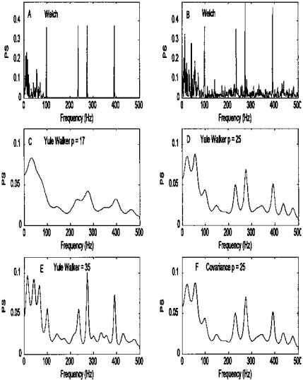
FIGURE 5.2 Comparison of AR and classical spectral analysis on a complex spectrum. (A) Spectrum obtained using classical methods (Welch) of a waveform consisting of four sinusoids (100, 240, 280, and 400 Hz) and a low frequency region generated from lowpass filtered noise. (B) Spectrum obtained using the Welch method applied to the same waveform after white noise has been added (SNR = -8 db). (C, D and E) Spectra obtained using AR models (Yule-Walker) having three different model orders. The lower order model (p = 17) cannot distinguish the two closely spaced sinusoids (240 and 280 Hz). The highest order model (p = 35) better identifies the 100 Hz signal and shows sharper peaks, but shows spurious peaks in the low frequency range. (F) AR spectral analysis using the covariance method produces results nearly identical to the Yule-Walker method.

Copyright 2004 by Marcel Dekker, Inc. All Rights Reserved.

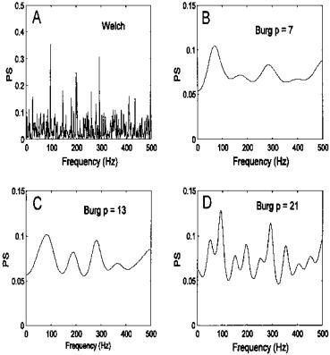
FIGURE 5.3 Spectra obtained from a waveform consisting of equal amplitude sinusoids at 100, 200, and 300 Hz with white noise (N = 1024; SNR = -12 db).

(A) The traditional Welch method shows the 3 sinusoids, but also lesser peaks due solely to the noise. (B) The AR method with low model order (p = 7) shows the two outside peaks with a hint of the center peak. (C) A higher order AR model (p = 13) shows the three peaks clearly. (D) An even higher order model (p = 21) shows the three peaks with better frequency resolution, but also shows a number of spurious peaks.

MATLAB Implementation

The four AR-based spectral analysis approaches described above are available in the MATLAB Signal Processing Toolbox. The AR routines are implemented though statements very similar in format to that used for the Welsh power spectral analysis described in Chapter 3. For example, to implement the Yule-Walker AR method the MATLAB statement would be:

Copyright 2004 by Marcel Dekker, Inc. All Rights Reserved.

[PS, freq] = pyulear(x,p,nfft,Fs);

Only the first two input arguments, x and p, are required as the other two have default values. The input argument, x, is a vector containing the input waveform, and p is the order of the AR model to be used. The input argument nfft specifies the length of the data segment to be analyzed, and if nfft is less than the length of x, averages will be taken as in pwelch. The default value for nfft is 256*. As in pwelch, Fs is the sampling frequency and if specified is used to appropriately fill the frequency vector, freq, in the output. This output variable can be used in plotting to obtain a correctly scaled frequency axis (see Example 5.1). In the AR spectral approach, Fs is also needed to scale the horizontal axis of the output spectrum correctly. If Fs is not specified, the output vector freq varies in the range of 0 to π.

As in routine pwelch, only the first output argument, PS, is required, and it contains the resultant power spectrum. Similarly, the length of PS is either (nfft/2) 1 if nfft is even, or (nfft 1)/2 if nfft is odd since additional points would be redundant. An exception is made if x is complex, in which case the length of PS is equal to nfft. Other optional arguments are available and are described in the MATLAB help file.

The other AR methods are implemented using similar MATLAB statements, differing only in the function name.

[Pxx, freq] = pburg(x,p,nfft,Fs); [Pxx, freq] = pcov(x,p,nfft,Fs); [Pxx, freq] = pmcov(x,p,nfft,Fs);

The routine pburg, uses the Burg method, pcov the covariance method and pmcov the modified covariance method. As we will see below, this general format is followed in other MATLAB spectral methods.

Example 5.1 Generate a signal combining lowpass filtered noise, four sinusoids, two of which are closely spaced, and white noise (SNR = -3 db). This example is used to generate the plots in Figure 5.2.

%Example 5.1 and Figure 5.2

%Program to evaluate different modern spectral methods

%Generate a spectra of lowpass filtered noise, sinusoids, and

%noise that applies classical and AR sprectral analysis methods

*Note the use of the term nfft is somewhat misleading since it implies an FFT is taken, and this is not the case in AR spectral analysis. We use it here to be consistent with MATLAB’s terminology.

Copyright 2004 by Marcel Dekker, Inc. All Rights Reserved.

% (25 Hz)

%

%Generate the low frequency broadband process

%Compute the impulse response of a Butterworth lowpass filter

%

% Generate the sinusoidal data and add to broadband signal [x,f,sig] = sig_noise([100 240 280 400],-8,N);

%Estimate the Welch spectrum using all points, no window, and no

%overlap

%Plot noiseless signal

[PS,f] = pwelch(sig,N,[ ],[ ],fs); subplot(3,2,1);

plot(f,PS,’k’); % Plot PS

.......labels, text, and axis .......

%

% Apply Welch method to noisy data set [PS,f] = pwelch(x, N,[ ],[ ],fs); subplot(3,2,2);

plot(f,PS,’k’);

%

% Apply AR to noisy data set at three different weights [PS,f] = pyulear(x,17,N,fs); % Yule-Walker; p = 17 subplot(3,2,3);

plot(f,PS,’k’);

Copyright 2004 by Marcel Dekker, Inc. All Rights Reserved.