Biosignal and Biomedical Image Processing MATLAB based Applications - John L. Semmlow

FIGURE 13.3 Example of back-projection on a simple 3-by-3 pixel grid. The upper grid represents the original image which contains a dark (absorption 8) center pixel surrounded by lighter (absorption 2) pixels. The projections are taken as the linear addition of all intervening pixels. In the lower reconstructed image, each pixel is set to the average of all beams that cross that pixel. (Normally the sum would be taken over a much larger set of pixels.) The center pixel is still higher in absorption, but the background is no longer the same. This represents a smearing of the original image.

frequency domain as the projection angle (Figure 13.6). Once the two-dimen- sional Fourier transform space is filled from the individual one-dimensional Fourier transforms of the projection profiles, the image can be constructed by applying the inverse two-dimensional Fourier transform to this space. Before the inverse transform is done, the appropriate filter can be applied directly in the frequency domain using multiplication.

As with other images, reconstructed CT images can suffer from alaising if they are undersampled. Undersampling can be the result of an insufficient

Copyright 2004 by Marcel Dekker, Inc. All Rights Reserved.

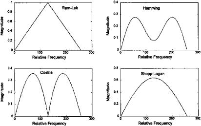
FIGURE 13.4 Magnitude frequency characteristics of four common filters used in filtered back-projection. They all show highpass characteristics at lower frequencies. The cosine filter has the same frequency characteristics as the two-point central difference algorithm.

number of parallel beams in the projection profile or too few rotation angles. The former is explored in Figure 13.7 which shows the square pattern of Figure 13.5 sampled with one-half (left-hand image) and one-quarter (right-hand image) the number of parallel beams used in Figure 13.5. The images have been multiplied by a factor of 10 to enhance the faint aliasing artifacts. One of the problems at the end of this chapter explores the influence of undersampling by reducing the number of angular rotations an well as reducing the number of parallel beams.

Fan Beam Geometry

For practical reasons, modern CT scanners use fan beam geometry. This geometry usually involves a single source and a ring of detectors. The source rotates around the patient while those detectors in the beam path acquire the data. This allows very high speed image acquisition, as short as half a second. The source fan beam is shaped so that the beam hits a number of detections simultaneously, Figure 13.8. MATLAB provides several routines that provide the Radon and inverse Radon transform for fan beam geometry.

Copyright 2004 by Marcel Dekker, Inc. All Rights Reserved.

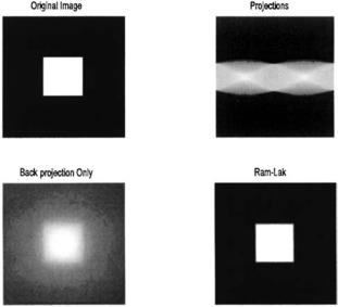
FIGURE 13.5 Image reconstruction of a simple white square against a black background. Back-projection alone produces a smeared image which can be corrected with a spatial derivative filter. These images were generated using the code given in Example 13.1.

MATLAB Implementation

Radon Transform

The MATLAB Image Processing Toolbox contains routines that perform both the Radon and inverse Radon transforms. The Radon transform routine has already been introduced as an implementation of the Hough transform for straight line objects. The procedure here is essentially the same, except that an intensity image is used as the input instead of the binary image used in the Hough transform.

[p, xp] = radon(I, theta);

where I is the image of interest and theta is the production angle in degs.s, usually a vector of angles. If not specified, theta defaults to (1:179). The output parameter p is the projection array, where each column is the projection profile at a specific angle. The optional output parameter, xp gives the radial coordinates for each row of p and can be used in displaying the projection data.

Copyright 2004 by Marcel Dekker, Inc. All Rights Reserved.

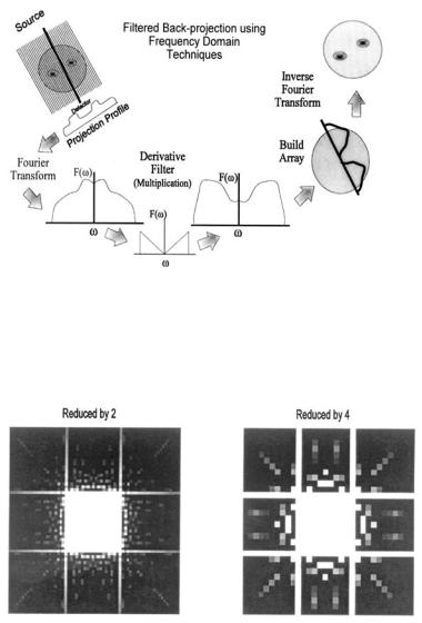
FIGURE 13.6 Schematic representation of the steps in filtered back-projection using frequency domain techniques. The steps shown are for a single projection profile and would be repeated for each projection angle.

FIGURE 13.7 Image reconstructions of the same simple pattern shown in Figure 13.4, but undersampled by a factor of two (left image) or four (right image). The contrast has been increased by a factor of ten to enhance the relatively lowintensity aliasing patterns.

Copyright 2004 by Marcel Dekker, Inc. All Rights Reserved.

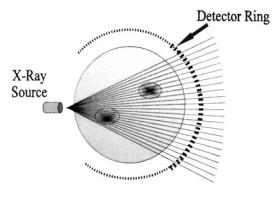
FIGURE 13.8 A series of beams is projected from a single source in a fan-like pattern. The beams fall upon a number of detectors arranged in a ring around the patient. Fan beams typically range between 30 to 60 deg. In the most recent CT scanners (so-called fourth-generation machines) the detectors completely encircle the patient, and the source can rotate continuously.

Inverse Radon Transform: Parallel Beam Geometry

MATLAB’s inverse Radon transform is based on filtered back-projection and uses the frequency domain approach illustrated in Figure 13.6. A variety of filtering options are available and are implemented directly in the frequency domain.

The calling structure of the inverse Radon transform is:

[I,f] = iradon(p,theta,interp,filter,d,n);

where p is the only required input argument and is a matrix where each column contains one projection profile. The angle of the projection profiles is specified by theta in one of two ways: if theta is a scalar, it specifies the angular spacing (in degs.s) between projection profiles (with an assumed range of zero to number of columns − 1); if theta is a vector, it specifies the angles themselves, which must be evenly spaced. The default theta is 180 deg. divided by the number of columns. During reconstruction, iradon assumes that the center of rotation is half the number of rows (i.e., the midpoint of the projection profile: ceil(size (p,1)/2)).

The optional argument interp is a string specifying the back-projection interpolation method: ‘nearest’, ‘linear’ (the default), and ‘spline’. The

Copyright 2004 by Marcel Dekker, Inc. All Rights Reserved.

filter option is also specified as a string. The ‘Ram-Lak’ option is the default and consists of a ramp in frequency (i.e., an ideal derivative) up to some maximum frequency (Figure 13.4 (on p. 382)). Since this filter is prone to highfrequency noise, other options multiply the ramp function by a lowpass function. These lowpass functions are the same as described above: Hamming window (‘Hamming’), Hanning window (‘Hann’), cosine (‘cosine’), and sinc (‘Shepp-Logan’) function. Frequency plots of several of these filters are shown in Figure 13.4. The filter’s frequency characteristics can be modified by the optional parameter, d, which scales the frequency axis: if d is less than one (the default value is one) then filter transfer function values above d, in normalized frequency, are set to 0. Hence, decreasing d increases the lowpass filter effect. The optional input argument, n, can be reused to rescale the image. These filter options are explored in several of the problems.

The image is contained in the output matrix I (class double), and the optional output vector, h, contains the filter’s frequency response. (This output vector was used to generate the filter frequency curves of Figure 13.4.) An application of the inverse Radon transform is given in Example 13.1.

Example 13.1 Example of the use of back-projection and filtered backprojection. After a simple image of a white square against a dark background is generated, the CT projections are constructed using the forward Radon transform. The original image is reconstructed from these projections using both the filtered and unfiltered back-projection algorithm. The original image, the projections, and the two reconstructed images are displayed in Figure 13.5 on page 385.

%Example 13.1 and Figure 13.4.

%Image Reconstruction using back-projection and filtered

%back-projection.

%Uses MATLAB’s ‘iradon’ for filtered back-projection and

%‘i_back’ for unfiltered back-projection.

%(This routine is a version of ‘iradon’ modified to eliminate

%the filter.)

%Construct a simple image consisting of a white square against

%a black background. Then apply back-projection without

%filtering and with the derivative (Ram-Lak) filters.

%Display the original and reconstructed images along with the

%projections.

%

clear all; close all;

%

I = zeros(128,128); I(44:84,44:84) = 1;

Copyright 2004 by Marcel Dekker, Inc. All Rights Reserved.

%

% Generate the projections using ‘radon’

theta = (1:180); % Angle between projections

% is 1 deg.

The display generated by this code is given in Figure 13.4. Example 13.2 explores the effect of filtering on the reconstructed images.

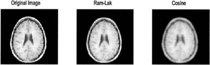
Example 13.2 The inverse Radon transform filters. Generate CT data by applying the Radon transform to an MRI image of the brain (an unusual example of mixed modalities!). Reconstruct the image using the inverse Radon transform with the Ram-Lak (derivative) filter and the cosine filter with a maximum relative frequency of 0.4. Display the original and reconstructed images.

%Example 13.2 and Figure 13.9 Image Reconstruction using

%filtered back-projection

%Uses MATLAB’s ‘iradon’ for filtered backprojection

%Load a frame of the MRI image (mri.tif) and construct the CT

%projections using ‘radon’. Then apply backprojection with

%two different filters: Ram-Lak and cosine (with 0.4 as

%highest frequency

% image

end

I = im2double(I); % Convert to double and scale

%

% Construct projections of MR image delta_theta = (1:180);

[p,xp] = radon(I,delta_theta); % Angle between projections

% is 1 deg.

Copyright 2004 by Marcel Dekker, Inc. All Rights Reserved.

%

% Reconstruct image using Ram-Lak filter I_RamLak = iradon(p,delta_theta,‘Ram-Lak’);

%

.......Display images.......

Radon and Inverse Radon Transform: Fan Beam Geometry

The MATLAB routines for performing the Radon and inverse Radon transform using fan beam geometry are termed fanbeam and ifanbeam, respectively, and have the form:

fan = fanbeam(I,D)

where I is the input image and D is a scalar that specifies the distance between the beam vertex and the center of rotation of the beams. The output, fan, is a matrix containing the fan bean projection profiles, where each column contains the sensor samples at one rotation angle. It is assumed that the sensors have a one-deg. spacing and the rotation angles are spaced equally over 0 to 359 deg. A number of optional input variables specify different geometries, sensor spacing, and rotation increments.

The inverse Radon transform for fan beam projections is specified as:

I = ifanbeam(fan,D)

FIGURE 13.9 Original MR image and reconstructed images using the inverse Radon transform with the Ram-Lak derivative and the cosine filter. The cosine filter’s lowpass cutoff has been modified by setting its maximum relative frequency to 0.4. The Ram-Lak reconstruction is not as sharp as the original image and sharpness is reduced further by the cosine filter with its lowered bandwidth. (Original image from the MATLAB Image Processing Toolbox. Copyright 1993– 2003, The Math Works, Inc. Reprinted with permission.)

Copyright 2004 by Marcel Dekker, Inc. All Rights Reserved.

where fan is the matrix of projections and D is the distance between beam vertex and the center of rotation. The output, I, is the reconstructed image. Again there are a number of optional input arguments specifying the same type of information as in fanbeam. This routine first converts the fan beam geometry into a parallel geometry, then applies filtered back-projection as in iradon. During the filtered back-projection stage, it is possible to specify filter options as in iradon. To specify, the string ‘Filter’ should precede the filter name (‘Hamming’, ‘Hann’, ‘cosine’, etc.).

Example 13.3 Fan beam geometry. Apply the fan beam and parallel beam Radon transform to the simple square shown in Figure 13.4. Reconstruct the image using the inverse Radon transform for both geometries.

%Example 13.3 and Figure 13.10

%Example of reconstruction using the Fan Beam Geometry

%Reconstructs a pattern of 4 square of different intensities

%using parallel beam and fan beam approaches.

I(76:106,76:106) = 1;

%

%Construct projections: Fan and parallel beam [F,Floc,Fangles] = fanbeam (I,D,‘FanSensorSpacing’,.5);

[R,xp] = radon(I,theta);

%Reconstruct images. Use Shepp-Logan filter

I_rfb = ifanbeam(F,D,‘FanSensorSpacing’,.5,‘Filter’, ...

‘Shepp-Logan’);

I_filter_back = iradon(R,theta,‘Shepp-Logan’);

%

% Display images subplot(1,2,1);

imshow(I_rfb); title(‘Fan Beam’) subplot(1,2,2);

imshow(I_filter_back); title(‘Parallel Beam’)

Copyright 2004 by Marcel Dekker, Inc. All Rights Reserved.

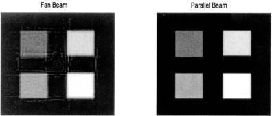
The images generated by this example are shown in Figure 13.10. There are small artifacts due to the distance between the beam source and the center of rotation. The affect of this distance is explored in one of the problems.

MAGNETIC RESONANCE IMAGING

Basic Principles

MRI images can be acquired in a number of ways using different image acquisition protocols. One of the more common protocols, the spin echo pulse sequence, will be described with the understanding that a fair number of alternatives are commonly used. In this sequence, the image is constructed on a slice-by-slice basis, although the data are obtained on a line-by-line basis. For each slice, the raw MRI data encode the image as a variation in signal frequency in one dimension, and in signal phase in the other. To reconstruct the image only requires the application of a two-dimensional inverse Fourier transform to this frequency/phase encoded data. If desired, spatial filtering can be implemented in the frequency domain before applying the inverse Fourier transform.

The physics underlying MRI is involved and requires quantum mechanics for a complete description. However, most descriptions are approximations that use classical mechanics. The description provided here will be even more abbreviated than most. (For a detailed classical description of the MRI physics see Wright’s chapter in Enderle et al., 2000.). Nuclear magnetism occurs in nuclei with an odd number of nucleons (protons and/or neutrons). In the presence of a magnetic field such nuclei possess a magnetic dipole due to a quantum mechani-

FIGURE 13.10 Reconstruction of an image of four squares at different intensities using parallel beam and fan beam geometry. Some artifact is seen in the fan beam geometry due to the distance between the beam source and object (see Problem 3).

Copyright 2004 by Marcel Dekker, Inc. All Rights Reserved.