

Biomolecular Sensing Processing and Analysis - Rashid Bashir and Steve Wereley
.pdf360 |
D. FOURGUETTE, E. ARIK, AND D. WILSON |
|
Spalding Formula |
Re=0.38E6 |
Re=0.69E6 |
|
|
Re=0.84E6 |
Re=1.11E6 |
Re=1.52E6 |
|
|
Linear sublayer |
Logarithmic Overlap |
Re=3.18E6 |
|
|
Re=4.45E6 |
Re=5.71E6 |
|
|
30 |
|
|
|
|
25 |
|
|
|
|
20 |
|
|
|
|
τ |
|
|
|
|
u/ u |
|
|
|
|
15 |
|
|
|
|
= |
|
|
|
|
+ |
|
|
|
|
u |
|
|
|
|
10 |
|
|
|
|
5 |
|
|
|
|
0 |
|
|
|
|
0.1 |
1.0 |
10.0 |
100.0 |
1000.0 |
|
|
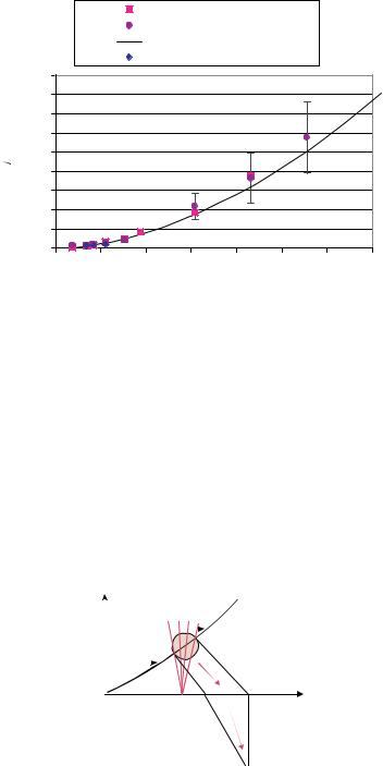
y+ = y uτ / ν |
|
|
FIGURE 17.11. Spalding fit to dual velocity measurements using the Dual Velocity sensor.
beam lithography using 0.25 mm square pixels and 64 depth levels. As a result, the two peaks in the signal are well defined and the processing yields a data rate 4 times higher than in previous velocity sensors.
The Dual Micro Velocimeter was tested in the flat plate boundary layer in a water tunnel. The wall shear stress was calculated from the dual velocity measurements using a Spalding fit through the linear sub-layer and the logarithmic overlap. Figure 17.11 shows the Spalding fit to five sets of dual velocity measurements in the sub-layer.
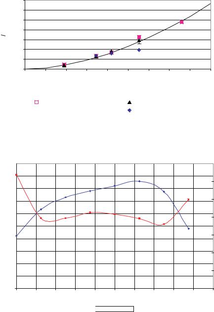
The wall shear stress measurements obtained using the Dual Velocity sensor are shown in Figure 17.12, combined with the results from the boundary layer survey obtained with the Mini LDV. These results show that the dual velocity approach to measure wall shear stress performs very well at Reynolds number in excess of 5.5 million and is a viable extension to the Diverging Doppler sensor.
17.5.2.2. Diverging Fringe Doppler Sensor The Doppler shear stress sensor, the MicroS3TM developed for this experiment is based on a technique first presented by Naqwi and Reynolds [17] using conventional optics. They projected a set of diverging fringe pattern and used the Doppler shift to measure the gradient of the flow velocity at the wall.
This sensor measures the flow velocity within the first 100 micrometers of the sensor surface. The optical probe volume extends over 30 µm. In this region of steep velocity gradient, the probe volume is designed to measure velocity over the 30 µm span by using diverging Doppler fringes (as opposed to parallel fringes in conventional Doppler sensors).
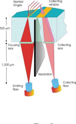
Figure 17.13 shows a schematic of the optical MEMS sensor principle. Diverging interference fringes originate at the surface and extend into the flow. The scattered light from the particle passing through the fringes is collected through a window at the surface
362 |
D. FOURGUETTE, E. ARIK, AND D. WILSON |
FIGURE 17.14. Schematic of the Diverging Fringe Doppler sensor.
which is equal to the wall shear,
σ = µ ∂ y w |
≡ µ y |
(17.2) |
∂u |
u |
|
in the linear sub-layer region of the boundary layer.
A schematic of the Diverging Fringe Doppler sensor is shown in Figure 17.14. A single mode emitting fiber illuminates a focusing lens (DOE shown in Figure 17.2) that shapes the light into two elongated beams of light. These two elongated beams of light are passed through a pair of slits to create two diffractive patterns. The interference between these diffractive patterns generates a set of diverging fringes originating at the sensor surface. The scattered light collected from the particles intersecting the probe volume is collected through window at the sensor surface and imaged into a collecting fiber with a second DOE. A detector pigtailed to the collecting fiber converts the optical burst into a signal.
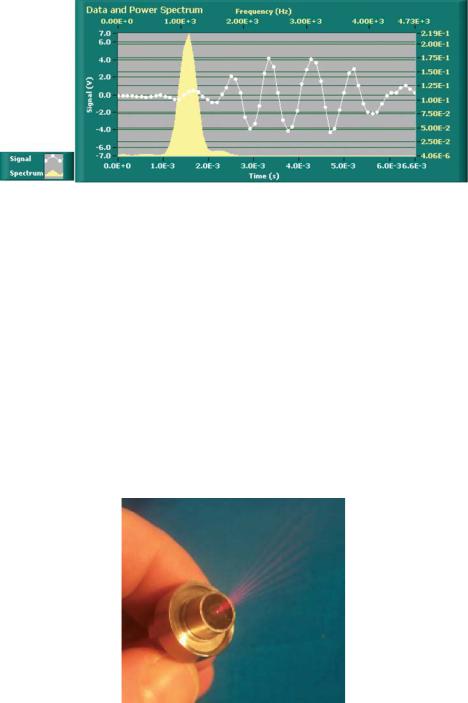
Figure 17.15 shows a plot of a burst obtained with the Diverging Fringe Doppler sensor (white trace) and the frequency spectrum of the burst obtained with an FFT (yellow filled trace). The signal conditioning and processing required for the shear stress sensor is identical to those used for a laser Doppler velocimeter. The burst was previously high-pass filtered to eliminate the low frequency pedestal and low-pass filtered to eliminate high frequency noise.
A photograph of the shear stress sensor is shown in Figure 17.16. The sensor chip, 4 mm × 4 mm, is mounted into the sensor element location shown on the front face of the assembly. The diverging fringe pattern is illuminated with the help of a fogger.

 Ubar
Ubar 
 U'/Ubar
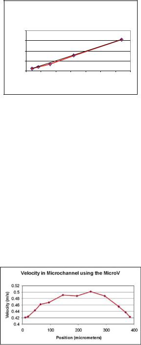
366 |
D. FOURGUETTE, E. ARIK, AND D. WILSON |
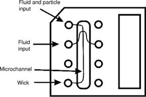
FIGURE 17.21. Schematic of the Caliper microfluidic chip.
between cells 10 µm and 20 µm in size, and also between single and paired cells 10 um in size.
Tests conducted at Caliper showed that cells 10 um in size in a buffer solution could be detected with VioSense’s MicroVTM, albeit with a low signal to noise ratio. The low signal to noise ratio was attributed in part to a large DC offset caused by light reflection at the surface of the chip. Additional measurements were needed to determine the origin of the light reflections and also the optical distortion sustained by the probe volume within the microchannel.
17.6.2.1.Experimental Setup A schematic of the microchannel, supplied by Caliper, is provided in Figure 17.21. The microchannel is 75 um wide and 25 um deep with a gutter type profile at the bottom. The chip material is glass. Distilled water containing particles
6.3um in size was dropped in the upper left well while distilled water was dropped in the fluid input ports. Lens paper was used to wick the fluid through the channel.
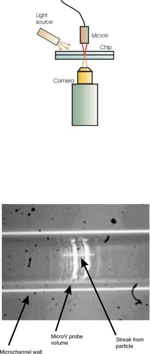
A schematic of the experimental setup is shown in Figure 17.22. A microscope objective and a camera were placed under the chip and an OEM version of the MicroVTM was placed above the chip. The camera was used to position the MicroV probe volume into the microchannel. A broadband light source was used to illuminate the chip. The light refracted by the channel walls helped identify the location of the microchannel.
Figure 17.23 shows a photograph of the microchannel with the MicroVTM probe volume position. The light source was positioned such that the microchannel walls are seen as the two bright lines across the photograph. The probe volume is visible as the two slightly curved vertical lines but is still clearly defined. The streak across the probe volume is caused by a particle traveling through the probe volume at the time the frame was acquired. Some distortion and optical reflections of the probe volume by the microchannel walls are visible in the photograph.
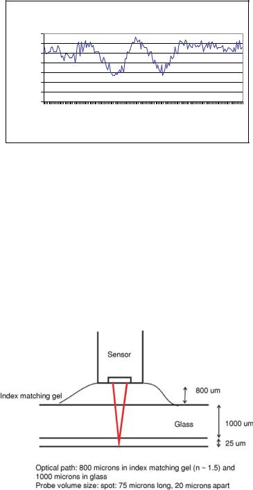
17.6.2.2.Results Time traces of the light intensity were acquired using a digital scope and one of the traces is displayed in Figure 17.24. The scattered light from the surfaces generates a DC contribution of 7.5 volts on the detector (out of 10 volts, the saturation
OPTICAL MEMS-BASED SENSOR DEVELOPMENT WITH APPLICATIONS TO MICROFLUIDICS 369
The sensor would be designed with a working distance of 1.8 mm in glass or in a material with equivalent index of refraction. The 0.8 mm layer of index matching gel is used to minimize the reflections off the upper glass surface while still allowing vertical adjustment for probe positioning. Coupling gel reduces unwanted scattering off the glass surfaces by up to 75%.
17.7. CONCLUSIONS
Recent advances in optical MEMS technology have enabled the development of diffractive optical elements capable of generating complex optical probe volume configurations. This optical MEMS technology is the enabling factor in the development and fabrication of optical microsensors. These microsensors provide the ability to precisely control the shape and location of the optical probe volume and provide reliable optical alignment, requirements that are necessary for optical diagnostics in microfluidic environments. Preliminary tests have yielded encouraging results towards the possibility of using these optical microsensors for fluid flow characterization for microfluidics applications.
BIBLIOGRAPHY
[1]E. Arik. Current status of particle image velocimetry and laser doppler anemometry instrumentation. In R.J. Donnelly and K.R. Sreenivasan (eds.), Flow at Ultra-High Reynolds and Rayleigh Numbers. Springer-Verlag, NY, 1998.
[2]W. Bachalo. Method for measuring the size and velocity of spheres by Dual-beam light-scatter interferometry. Appl. Optics, 3:363, 1980.
[3]D. Dopheide, M. Faber, Y. Bing, and G. Taux. Semiconductor long-range anemometer using a 5 mW diode laser and a pin photodiode. In R.J Adrian (ed.), Applications of Laser Techniques to Fluid Mechanics, Springer-Verlag, pp. 385–399, 1990.
[4]F. Durst, A. Melling, and J.H. Whitelaw. Principles and Practice of Laser Doppler Anemometry. Academic Press 1976.
[5]D. Fourguette, D. Modarress, D. Wilson, M. Koochesfahani, and M. Gharib. An Optical MEMS-based Shear Stress Sensor for High Reynolds Number Applications. AIAA Paper 2003–0742, 41st AIAA Aerospace Sciences Meeting & Exhibit, Reno, NV, 2003.
[6]D. Fourguette, D. Modarress, F. Taugwalder, D. Wilson, M. Koochesfahani, and M. Gharib. Miniature and MOEMS Flow Sensors. Paper AIAA-2001-2982, 31st Fluid Dynamics Conference & Exhibit Anaheim, CA, 2001.
[7]D. Fourguette and C. Suarez. Integrated Optical Diagnostics for Miniature Devices. AIAA Paper 99-0514, 37th AIAA Aerospace Sciences Meeting & Exhibit, Reno, NV, 1999.
[8]M. Gharib, D. Modarress, D. Fourguette, and D. Wilson. Optical Microsensors for Fluid Flow Diagnostics.
AIAA Paper 2002–0252, 40th AIAA Aerospace Sciences Meeting & Exhibit, Reno, NV, 2002.
[9]R.W. Gerchberg and W.O. Saxton. A practical algorithm for the determination of phase from images and diffraction plane pictures, Optik, 35:237–246, 1972.
[10]M. Johansson and J. Bengtsson. Robust design method for highly efficient beam-shaping diffractive optical elements using an iterative-fourier-transform algorithm with soft operations. J. Mod. Opt., 47:1385–1398, 2000.
[11]B. Lehmann, C. Hassa, and J. Helbig. Three-component laser-doppler measurements of the confined model flow behind a swirl nozzle. Developments if Laser Techniques and Fluid Mechanics, Selected Papers from the 8th International Symposium, Lisbon, Portugal, Springer Press, pp. 383–398, 1996.
[12]P.D. Maker and R.E. Muller. Phase holograms in polymethylmethacrylate. J. Vac. Sci. Tech. B, 10:2516–2519, 1992.