

Universal Serial Bus Specification Revision 1.1
5.10.2 USB Clock Model
Time is present in the USB system via clocks. In fact, there are multiple clocks in a USB system that must be understood:
Sample Clock: This clock determines the natural data rate of samples moving between client software on the host and the function. This clock does not need to be different between non-USB and USB implementations.
Bus Clock: This clock runs at a 1.000ms period (1kHz frequency) and is indicated by the rate of SOF packets on the bus. This clock is somewhat equivalent to the 8MHz clock in the non-USB example. In the USB case, the bus clock is often a lower-frequency clock than the sample clock, whereas the bus clock is almost always a higher-frequency clock than the sample clock in a non-USB case.
Service Clock: This clock is determined by the rate at which client software runs to service IRPs that may have accumulated between executions. This clock also can be the same in the USB and non-USB cases.
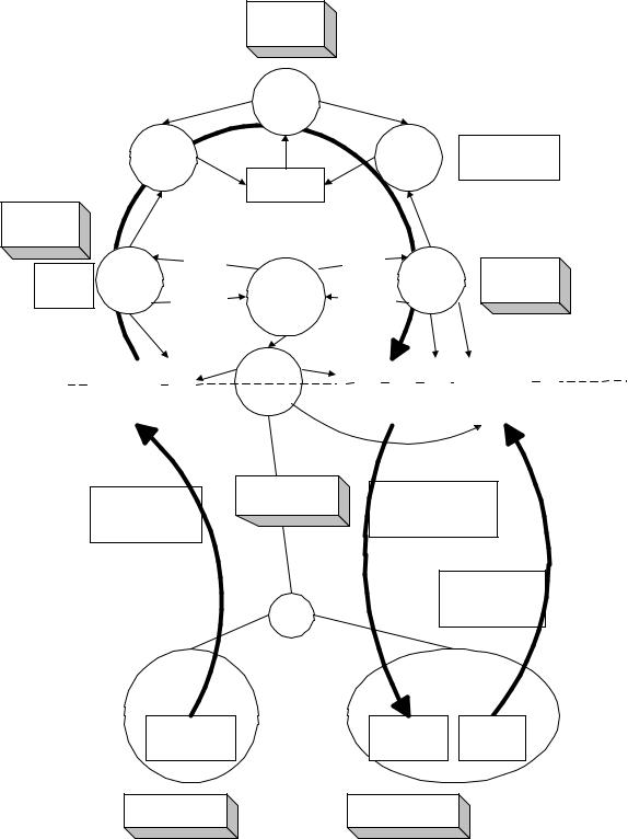
In most existing operating systems, it is not possible to support a broad range of isochronous communication flows if each device driver must be interrupted for each sample for fast sample rates. Therefore, multiple samples, if not multiple packets, will be processed by client software and then given to the Host Controller to sequence over the bus according to the prenegotiated bus access requirements. Figure 5-14 presents an example for a reasonable USB clock environment equivalent to the non-USB example in Figure 5-13.
59
Universal Serial Bus Specification Revision 1.1
Each DD has independent service rate
Mixer Device
Driver
|
|
1 speaker DD |
Rate |
Rate |
service period |
Matcher |
Matcher |
(n sample) |
|
Master Clock |
slop buffer |
|
|
20ms service period
|
|
Transfer |
|
Transfer |
|
|
|
|
Complete |
|
|
|
|
|
|
|
Complete |
|
|
|
|
|
Interrupt |
|
|
|
|
|
Microphone |
|
Interrupt |
Speaker |
20ms service |
|
1 sample |
|
|
||||
Device Driver |
|
|
|
Device Driver |
period |
|
slop buffer |
|
US B SW |
|
|||
|
QueueBuffer |
QueueBuffer |
|
|
||
|
|
|
|
2x161 Byte Buffer |
Host |
2x3532 |
Byte Buffer |
|
1x3 Byte Buffer |
|
Software |
(2 Services, |
|
(2 Services, |
|
|
|||
|
|
(1 Services, |
|
Hardware |
|||
159-161 samples per |
Controller |
881-883 |
samples per |
|
|
||
|
1 feedback per service |
|
|
||||
service, |
|
service |
|
|
|
||
|
|
1 packets/service) |
|
|
|||
20 packets/service) |
|
20 packets/service) |
|
|
|
||
|
|
|
|
|
|||
|
|
|
|
|
|
|
|
1KHz Bus Clock
7-9 Byte Packets
172-184 Byte Packets
7-9 samples per packet
43-46 samples per packet
3 byte packets Feedback Info
Hub
Mono |
|
CD Stereo |
|
Microphone |
|
Speakers |
|
8+9 Byte Buffer |
(44+45+1+1)x4 |
1x3 Byte |
|
Byte Buffer |
Buffer |
||
(2 Packets) |
|||
(2 Packets) |
(1 Packets) |
||
|
8kHz Sample Clock (1 byte/sample)
44.1KHz Sample Clock
(4 bytes/sample)
Figure 5-14. USB Isochronous Application
60
Universal Serial Bus Specification Revision 1.1
Figure 5-14 shows a typical round trip path of information from a microphone as an input device to a speaker as an output device. The clocks, packets, and buffering involved are also shown. Figure 5-14 will be explored in more detail in the following sections.
The focus of this example is to identify the differences introduced by the USB compared to the previous non-USB example. The differences are in the areas of buffering, synchronization given the existence of a USB bus clock, and delay. The client software above the device drivers can be unaffected in most cases.
5.10.3 Clock Synchronization
In order for isochronous data to be manipulated reliably, the three clocks identified above must be synchronized in some fashion. If the clocks are not synchronized, several clock-to-clock attributes can be present that can be undesirable:
Clock Drift: Two clocks that are nominally running at the same rate can, in fact, have implementation differences that result in one clock running faster or slower than the other over long periods of time. If uncorrected, this variation of one clock compared to the other can lead to having too much or too little data when data is expected to always be present at the time required.
Clock Jitter: A clock may vary its frequency over time due to changes in temperature, etc. This may also alter when data is actually delivered compared to when it is expected to be delivered.
Clock-to-clock Phase Differences: If two clocks are not phase locked, different amounts of data may be available at different points in time as the beat frequency of the clocks cycle out over time. This can lead to quantization/sampling related artifacts.
The bus clock provides a central clock with which USB hardware devices and software can synchronize to one degree or another. However, the software will, in general, not be able to phaseor frequency-lock precisely to the bus clock given the current support for “real time-like” operating system scheduling support in most PC operating systems. Software running in the host can, however, know that data moved over the USB is packetized. For isochronous transfer types, a single packet of data is moved exactly once per frame and the frame clock is reasonably precise. Providing the software with this information allows it to adjust the amount of data it processes to the actual frame time that has passed.
5.10.4 Isochronous Devices
The USB includes a framework for isochronous devices that defines synchronization types, how isochronous endpoints provide data rate feedback, and how they can be connected together. Isochronous devices include sampled analog devices (for example, audio and telephony devices) and synchronous data devices. Synchronization type classifies an endpoint according to its capability to synchronize its data rate to the data rate of the endpoint to which it is connected. Feedback is provided by indicating accurately what the required data rate is, relative to the SOF frequency. The ability to make connections depends on the quality of connection that is required, the endpoint synchronization type, and the capabilities of the host application that is making the connection. Additional device class-specific information may be required, depending on the application.
Note: the term “data” is used very generally, and may refer to data that represents sampled analog information (like audio), or it may be more abstract information. “Data rate” refers to the rate at which analog information is sampled, or the rate at which data is clocked.
61
Universal Serial Bus Specification Revision 1.1
The following information is required in order to determine how to connect isochronous endpoints:
Synchronization type:
Asynchronous: Unsynchronized, although sinks provide data rate feedback
Synchronous: Synchronized to the USB’s SOF
Adaptive: Synchronized using feedback or feedforward data rate information
Available data rates
Available data formats.
Synchronization type and data rate information are needed to determine if an exact data rate match exists between source and sink, or if an acceptable conversion process exists that would allow the source to be connected to the sink. It is the responsibility of the application to determine whether the connection can be supported within available processing resources and other constraints (like delay). Specific USB device classes define how to describe synchronization type and data rate information.
Data format matching and conversion is also required for a connection, but it is not a unique requirement for isochronous connections. Details about format conversion can be found in other documents related to specific formats.
5.10.4.1 Synchronization Type
Three distinct synchronization types are defined. Table 5-7 presents an overview of endpoint synchronization characteristics for both source and sink endpoints. The types are presented in order of increasing capability.
Table 5-7. Synchronization Characteristics
|
Source |
Sink |
|
|
|
Asynchronous |
Free running Fs |
Free running Fs |
|
Provides implicit feedforward (data stream) |
Provides explicit feedback (interrupt pipe) |
|
|
|
Synchronous |
Fs locked to SOF |
Fs locked to SOF |
|
Uses implicit feedback (SOF) |
Uses implicit feedback (SOF) |
|
|
|
Adaptive |
Fs locked to sink |
Fs locked to data flow |
|
Uses explicit feedback (control pipe) |
Uses implicit feedforward (data stream) |
|
|
|
5.10.4.1.1 Asynchronous
Asynchronous endpoints cannot synchronize to SOF or any other clock in the USB domain. They source or sink an isochronous data stream at either a fixed data rate (single-frequency endpoints), a limited number of data rates (32kHz, 44.1kHz, 48kHz, …), or a continuously programmable data rate. If the data rate is programmable, it is set during initialization of the isochronous endpoint. Asynchronous devices must report their programming capabilities in the class-specific endpoint descriptor as described in their device class specification. The data rate is locked to a clock external to the USB or to a free-running internal clock. These devices place the burden of data rate matching elsewhere in the USB environment. Asynchronous source endpoints carry their data rate information implicitly in the number of samples they produce per frame. Asynchronous sink endpoints must provide explicit feedback information to an adaptive driver (refer to Section 5.10.4.2).
62
Universal Serial Bus Specification Revision 1.1
An example of an asynchronous source is a CD-audio player that provides its data based on an internal clock or resonator. Another example is a Digital Audio Broadcast (DAB) receiver or a Digital Satellite Receiver (DSR). Here too, the sample rate is fixed at the broadcasting side and is beyond USB control.
Asynchronous sink endpoints could be low-cost speakers, running off of their internal sample clock.
Another case arises when there are two or more devices present on the USB that need to have mastership control over SOF generation in order to operate as synchronous devices. This could happen if there were two telephony devices, each locked to a different external clock. One telephony device could be digitally connected to a Private Branch Exchange (PBX) that is not synchronized to the ISDN. The other device could be connected directly to the ISDN. Each device will source or sink data to/from the network side at an externally driven rate. Because only one of the devices can take mastership over the SOF, the other will sink or source data at a rate that is asynchronous to the SOF. This example indicates that every device capable of SOF mastership may be forced to operate as an asynchronous device.
5.10.4.1.2 Synchronous
Synchronous endpoints can have their clock system (their notion of time) controlled externally through SOF synchronization. These endpoints must be doing one of the following:
Slaving their sample clock to the 1ms SOF tick (by means of a programmable PLL).
Controlling the rate of USB SOF generation so that their data rate becomes automatically locked to SOF. In case these endpoints are not granted SOF mastership, they must degenerate to the asynchronous mode of operation (refer to the asynchronous example).
Synchronous endpoints may source or sink isochronous data streams at either a fixed data rate (singlefrequency endpoints), a limited number of data rates (32kHz, 44.1kHz, 48kHz, …), or a continuously programmable data rate. If programmable, the operating data rate is set during initialization of the isochronous endpoint. The number of samples or data units generated in a series of USB frames is deterministic and periodic. Synchronous devices must report their programming capabilities in the classspecific endpoint descriptor as described in their device class specification.
An example of a synchronous source is a digital microphone that synthesizes its sample clock from SOF and produces a fixed number of audio samples every USB frame. Another possibility is a 64kb/s bitstream from an ISDN “modem.” If the USB SOF generation is locked to the PSTN clock (perhaps through the same ISDN device), the data generation will also be locked to SOF and the endpoint will produce a stable 64kb/s data stream, referenced to the SOF time notion.
5.10.4.1.3 Adaptive
Adaptive endpoints are the most capable endpoints possible. They are able to source or sink data at any rate within their operating range. Adaptive source endpoints produce data at a rate that is controlled by the data sink. The sink provides feedback (refer to Section 5.10.4.2) to the source, which allows the source to know the desired data rate of the sink. Adaptive endpoints can communicate with all types of sink endpoints. For adaptive sink endpoints, the data rate information is embedded in the data stream. The average number of samples received during a certain averaging time determines the instantaneous data rate. If this number changes during operation, the data rate is adjusted accordingly.
The data rate operating range may center around one rate (e.g., 8kHz), select between several programmable or auto-detecting data rates (32kHz, 44.1kHz, 48kHz, …), or may be within one or more ranges (e.g., 5kHz to 12kHz or 44kHz to 49kHz). Adaptive devices must report their programming capabilities in the class-specific endpoint descriptor as described in their device class specification
An example of an adaptive source is a CD player that contains a fully adaptive sample rate converter (SRC) so that the output sample frequency no longer needs to be 44.1kHz but can be anything within the operating range of the SRC. Adaptive sinks include such endpoints as high-end digital speakers, headsets, etc.
63
Universal Serial Bus Specification Revision 1.1
5.10.4.2 Feedback
An asynchronous sink provides feedback to an adaptive source by indicating accurately what its desired data rate (Ff) is, relative to the USB SOF frequency. The required data rate is accurate to better than one sample per second (1Hz) in order to allow a high-quality source rate to be created and to tolerate delays and errors in the feedback loop.
The Ff value consists of a fractional part, in order to get the required resolution with 1kHz frames, and an integer part, which gives the minimum number of samples per frame. Ten bits are required to resolve one sample within a 1kHz frame frequency (1000 / 2^10 = 0.98). This is a ten-bit fraction, represented in unsigned fixed binary point 0.10 format. The integer part needs ten bits (2^10 = 1024) to encode up to 1,023 one-byte samples per frame. The ten-bit integer is represented in unsigned fixed binary point 10.0 format. The combined Ff value can be coded in unsigned fixed binary point 10.10 format, which fits into three bytes (24 bits). Because the maximum integer value is fixed to 1,023, the 10.10 number will be leftjustified in the 24 bits, so that it has a 10.14 format. Only the first ten bits behind the binary point are required. The lower four bits may be optionally used to extend the precision of Ff , otherwise, they shall be reported as zero. The bit and byte ordering follows the definitions of other multi-byte fields contained in Chapter 8.
Each frame, the adaptive source adds Ff to any remaining fractional sample count from the previous frame, sources the number of samples in the integer part of the sum, and retains the fractional sample count for the next frame. The source can look at the behavior of Ff over many frames to determine an even more accurate rate, if it needs to.
The sink can determine Ff by counting cycles of a clock with a frequency of Fs * 2^P for a period of 2^(10-P) frames, where P is an integer. P is practically bound to be in the range [0,10] because there is no point in using a clock slower than Fs, and no point in trying to update more than once a frame. The counter is read into Ff and reset every 2^(10-P) frames. As long as no clock cycles are skipped, the count will be accurate over the long term. An endpoint needs to implement only the number of counter bits that it requires for its maximum Ff.
A digital telephony endpoint, for example, will usually derive its 8kHz Fs by dividing down the 64kHz clock (P=3) which it uses to serialize the data stream. The 64kHz clock phase can also give an additional one bit of accuracy, effectively giving P=4. This would give Ff updates every 2^(10-4) = 64 frames. A 13bit counter would be required to obtain Ff, with three bits for eight samples per frame, and ten bits for the fractional part. The 13 bits would provide a 3.10 field within the 10.14 Ff value, with the remaining bits set to zero.
The choice of P is endpoint-specific. Use the following guidelines when choosing P:
P should be in the range [1,9].
Larger values of P are preferred, because they reduce the size of the frame counter and increase the rate at which Ff is updated. More frequent updates result in a tighter control of the source data rate, which reduces the buffer space required to handle Ff changes.
P should be less than ten so that Ff is averaged across at least two frames in order to reduce SOF jitter effects.
P should not be zero in order to keep the deviation in the number of samples sourced to less than 1 in the event of a lost Ff value.
Isochronous transfers are used to read Ff from the feedback register. The desired reporting rate for the feedback should be 2^(10-P) frames. Ff will be reported at most once per update period. There is nothing to be gained by reporting the same Ff value more than once per update period. The endpoint may choose to report Ff only if the updated value has changed from the previous Ff value.
It is possible that the source will deliver one too many or one too few samples over a long period, due to errors or accumulated inaccuracies in measuring Ff. The sink must have sufficient buffer capability to accommodate this. When the sink recognizes this condition, it should adjust the reported Ff value to
64
Universal Serial Bus Specification Revision 1.1
correct it. This may also be necessary to compensate for relative clock drifts. The implementation of this correction process is endpoint-specific and is not specified.
An adaptive source may obtain the sink data rate information from an adaptive sink that is locked to the same clock as the sink, as would be the case for a two-way speech connection. In this case, the feedback pipe is not needed.
5.10.4.3 Connectivity
In order to fully describe the source-to-sink connectivity process, an interconnect model is presented. The model indicates the different components involved and how they interact to establish the connection.
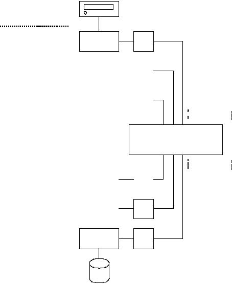
The model provides for multi-source/multi-sink situations. Figure 5-15 illustrates a typical situation (highly condensed and incomplete). A physical device is connected to the host application software through different hardware and software layers as described in the USB Specification. At the client interface level, a virtual device is presented to the application. From the application standpoint, only virtual devices exist. It is up to the device driver and client software to decide what the exact relation is between physical and virtual device.
65
Universal Serial Bus Specification Revision 1.1
Host Environment
CD-ROM
|
|
|
|
|
|
|
|
|
|
|
|
|
|
|
|
|
|
|
|
|
|
Device |
|
Client |
|
|
|
|
|
|
|
|
|
|
|
|
|
|
|
|
|
|
|
|
|
|
|
|
|
Physical Sources |
|
Driver |
|
|
|
|
|
|
|
|
|
|
|
|
|
|
|
|
|
|
|
|
|
|
|
|
|
||||||||||||||||||||
|
|
|
|
|
|
|
|
|
|
|
|
|
|
|
|
|
|
|
|
|
|
|
|
|
|
|
|
|||||||||||||||||||||
|
|
|
|
|
|
|
|
|
|
|
|
|
|
|
|
|
|
|
|
|
|
|
|
|
|
|
||||||||||||||||||||||
|
|
|
|
|
|
|
|
|
|
|
|
|
|
|
|
|
|
|
|
|
|
|
|
|
|
|
|
|
|
|
|
|
|
|
|
|
|
|
|
|
|
|
|
|
|
|
|
|
|
|
|
|
Source |
|
|
|
|
Isoc. Pipe |
Device |
|
Client |
|
|
|
|
|
|
|
|
|
|
|
|
|
|
|
|
|
|
|
|
|
|
|
|
||||||||||||
|
|
|
|
|
|
|
|
|
|
|
Driver |
|
|
|
|
|
|
|
|
|
|
|
|
|
|
|
|
|
|
|
|
|
|
|
|
|
||||||||||||
|
|
|
|
|
|
|
|
|
|
|
|
|
|
|
|
|
|
|
|
|
|
|
|
|
|
|
|
|
|
|
|
|
|
|
|
|
|
|
|
|
|
|
|
|
|
|
|
|
|
|
|
|
|
|
|
|
|
|
|
|
|
|
|
|
|
|
|
Isoc. Pipe |
|
|
|
|
|
|
|
|
|
|
|
|
|
|
|
|
|
|
|
|
|
|
|
|
|
|
|
||
|
|
|
|
|
|
|
|
|
|
|
|
|
|
|
|
|
|
|
|
|
|
|
|
|
|
|
|
|
|
|
|
|
|
|
|
|
|
|
|
|
|
|
|
|
|
|||
|
|
|
|
Source |
|
|
|
|
Device |
|
Client |
|
|
|
|
|
|
|
|
|
|
|
|
|
|
|
|
|
|
|
|
|
|
|
|
|||||||||||||
|
|
|
|
|
|
|
|
|
|
|
Driver |
|
|
|
|
|
|
|
|
|
|
|
|
|
|
|
|
|
|
|
|
|
|
|
|
|
||||||||||||
|
|
|
|
|
|
|
|
|
|
|
|
|
|
|
|
|
|
|
|
|
|
|
|
|
|
|
|
|
|
|
|
|
|
|
|
|
|
|
|
|
|
|
|
|
|
|
|
|
 Virtual Sources
USB Environment |
Application |
|
|
|
|
Virtual Sinks
|
|
|
|
|
|
|
Sink |
|
|
|
Isoc. Pipe |
Device |
|
Client |
|
|
|
|
|
|
|
|
|
|
|
|
|
|
|
|
|
|
|
|
|||||||||||||||
|
|
|
|
|
|
|
|
|
|
|
|
|
|
|
|
Driver |
|
|
|
|
|
|
|
|
|
|
|
|
|
|
|
|
|
|
|
|
|
||||||||||||
|
|
|
|
|
|
|
|
|
|
|
|
|
|
|
|
|
|
|
|
|
|
|
|
|
|
|
|
|
|
|
|
|
|
|
|
|
|
|
|
|
|
|
|
|
|
|
|
|
|
|
|
|
|
|
|
|
|
|
|
|
|
|
|
|
|
|
|
|
|
|
Isoc. Pipe |
|
|
|
|
|
|
|
|
|
|
|
|
|
|
|
|
|
|
|
|
|
|
|
|||||
|
|
|
|
|
|
|
|
|
|
|
|
|
|
|
|
|
|
|
|
|
|
|
|
|
|
|
|
|
|
|
|
|
|
|
|
|
|
|
|
|
|
|
|
||||||
|
|
|
|
|
|
|
Sink |
|
|
|
Device |
|
Client |
|
|
|
|
|
|
|
|
|
|
|
|
|
|
|
|
|
|
|
|
||||||||||||||||
|
|
|
|
|
|
|
|
|
|
|
|
|
|
|
|
Driver |
|
|
|
|
|
|
|
|
|
|
|
|
|
|
|
|
|
|
|
|
|
||||||||||||
|
|
|
|
|
|
|
|
|
|
|
|
|
|
|
|
|
|
|
|
|
|
|
|
|
|
|
|
|
|
|
|
|
|
|
|
|
|
|
|
|
|
|
|
|
|
|
|
|
|
|
|
|
|
|
|
|
|
|
|
|
|
|
|
|
|
|
|
|
|
|
|
|
|
|
|
|
|
|
|
|
|
|
|
|
|
|
|
|
|
|
|
|
|
|
|
|
|
|
|
|
|
|
|
|
|
|
|
|
|
|
|
|
|
|
|
|
|
|
|
|
|
|
|
|
|
|
Device |
|
|
|
|
|
|
|
|
|
|
|
|
|
|
|
|
|
|
|
|
|
|
|
|
Physical Sinks |
|
|
|
Client |
|
|
|
|
|
|
|
|
|
|
|
|
|
|
|
|
|
|
|
|
|||||||||||||||||||||||
|
|
|
|
|
|
|
|
|
|
|
|
|
|
|
|
|
|
|
|
|
|
|
|
||||||||||||||||||||||||||
|
|
|
|
|
|
|
|
|
|
|
|
|
|
|
|
|
|
|
|
|
|
|
|
||||||||||||||||||||||||||
|
|
|
|
|
|
|
|
|
|
|
|
|
|
|
|
|
|
|
|
|
|
|
|
|
|
|
|
|
|
|
|
|
|
|
|
|
|
|
|
|
|
|
|
|
|
|
|
|
|
Driver
Hard Disk
Figure 5-15. Example Source/Sink Connectivity
Device manufacturers (or operating system vendors) must provide the necessary device driver software and client interface software to convert their device from the physical implementation to a USB-compliant software implementation (the virtual device). As stated before, depending on the capabilities built into this software, the virtual device can exhibit different synchronization behavior from the physical device. However, the synchronization classification applies equally to both physical and virtual devices. All physical devices belong to one of the three possible synchronization types. Therefore, the capabilities that have to be built into the device driver and/or client software are the same as the capabilities of a physical device. The word “application” must be replaced by “device driver/client software.” In the case of a physical source to virtual source connection, “virtual source device” must be replaced by “physical source device” and “virtual sink device” must be replaced by “virtual source device.” In the case of a virtual sink
to physical sink connection, “virtual source device” must be replaced by “virtual sink device” and “virtual sink device” must be replaced by “physical sink device.”
66
Universal Serial Bus Specification Revision 1.1
Placing the rate adaptation (RA) functionality into the device driver/client software layer has the distinct advantage of isolating all applications, relieving the device from the specifics and problems associated with rate adaptation. Applications that would otherwise be multi-rate degenerate to simpler mono-rate systems.
Note: the model is not limited to only USB devices. For example, a CD-ROM drive containing 44.1kHz audio can appear as either an asynchronous, synchronous, or adaptive source. Asynchronous operation means that the CD-ROM fills its buffer at the rate that it reads data from the disk, and the driver empties the buffer according to its USB service interval. Synchronous operation means that the driver uses the USB service interval (e.g., 10ms) and nominal sample rate of the data (44.1kHz) to determine to put out 441 samples every USB service interval. Adaptive operation would build in a sample rate converter to match the CD-ROM output rate to different sink sampling rates.
Using this reference model, it is possible to define what operations are necessary to establish connections between various sources and sinks. Furthermore, the model indicates at what level these operations must or can take place. First there is the stage where physical devices are mapped onto virtual devices and vice versa. This is accomplished by the driver and/or client software. Depending on the capabilities included in this software, a physical device can be transformed into a virtual device of an entirely different synchronization type. The second stage is the application that uses the virtual devices. Placing rate matching capabilities at the driver/client level of the software stack relieves applications communicating with virtual devices from the burden of performing rate matching for every device that is attached to them. Once the virtual device characteristics are decided, the actual device characteristics are not any more interesting than the actual physical device characteristics of another driver.
As an example, consider a mixer application that connects at the source side to different sources, each running at their own frequencies and clocks. Before mixing can take place, all streams must be converted to a common frequency and locked to a common clock reference. This action can be performed in the physical-to-virtual mapping layer or it can be handled by the application itself for each source device independently. Similar actions must be performed at the sink side. If the application sends the mixed data stream out to different sink devices, it can either do the rate matching for each device itself or it can rely on the driver/client software to do that, if possible.
Table 5-8 indicates at the intersections what actions the application must perform to connect a source endpoint to a sink endpoint.
67
Universal Serial Bus Specification Revision 1.1
Table 5-8. Connection Requirements
|
|
Source Endpoint |
|
|
|
|
|
Sink Endpoint |
Asynchronous |
Synchronous |
Adaptive |
|
|
|
|
Asynchronous |
Async Source/Sink RA |
Async SOF/Sink RA |
Data + Feedback |
|
See Note 1. |
See Note 2. |
Feedthrough |
|
|
|
See Note 3. |
|
|
|
|
Synchronous |
Async Source/SOF RA |
Sync RA |
Data Feedthrough + |
|
See Note 4. |
See Note 5. |
Application Feedback |
|
|
|
See Note 6. |
|
|
|
|
Adaptive |
Data Feedthrough |
Data Feedthrough |
Data Feedthrough |
|
See Note 7. |
See Note 8. |
See Note 9. |
|
|
|
|
Notes:
1.Asynchronous RA in the application. Fsi is determined by the source, using the feedforward information embedded in the data stream. Fso is determined by the sink, based on feedback information from the sink. If nominally Fsi = Fso, the process degenerates to a feedthrough connection if slips/stuffs due to lack of synchronization are tolerable. Such slips/stuffs will cause audible degradation in audio applications.
2.Asynchronous RA in the application. Fsi is determined by the source but locked to SOF. Fso is determined by the sink, based on feedback information from the sink. If nominally Fsi = Fso, the process degenerates to a feedthrough connection if slips/stuffs due to lack of synchronization are tolerable. Such slips/stuffs will cause audible degradation in audio applications.
3.If Fso falls within the locking range of the adaptive source, a feedthrough connection can be established. Fsi = Fso and both are determined by the asynchronous sink, based on feedback information from the sink. If Fso falls outside the locking range of the adaptive source, the adaptive source is switched to synchronous mode and Note 2 applies.
4.Asynchronous RA in the application. Fsi is determined by the source. Fso is determined by the sink and locked to SOF. If nominally Fsi = Fso, the process degenerates to a feedthrough connection if slips/stuffs due to lack of synchronization are tolerable. Such slips/stuffs will cause audible degradation in audio applications.
5.Synchronous RA in the application. Fsi is determined by the source and locked to SOF. Fso is determined by the sink and locked to SOF. If Fsi = Fso, the process degenerates to a loss-free feedthrough connection.
6.The application will provide feedback to synchronize the source to SOF. The adaptive source appears to be a synchronous endpoint and Note 5 applies.
7.If Fsi falls within the locking range of the adaptive sink, a feedthrough connection can be established. Fsi = Fso and both are determined by and locked to the source.
If Fsi falls outside the locking range of the adaptive sink, synchronous RA is done in the host to provide an Fso that is within the locking range of the adaptive sink.
8.If Fsi falls within the locking range of the adaptive sink, a feedthrough connection can be established. Fso = Fsi and both are determined by the source and locked to SOF.
If Fsi falls outside the locking range of the adaptive sink, synchronous RA is done in the host to provide an Fso that is within the locking range of the adaptive sink.
9.The application will use feedback control to set Fso of the adaptive source when the connection is set up. The adaptive source operates as an asynchronous source in the absence of ongoing feedback information and Note 7 applies.
68